Welcome to the documentation for spheres!
spheres
toolbox for higher spin and symmetrization


spheres provides tools for dealing with higher spin systems and for symmetrized quantum circuits. Among other things, we provide implementations of:
The “Majorana stars” representation of a spin-j state as a degree-2j complex polynomial defined on the extended complex plane (the Riemann sphere). The eponymous stars are the 2j roots of this polynomial and each can be interpreted as a quantum of angular momentum contributing 1/2 in the specified direction. This polynomial can be defined in terms of the components of a
|j, m>vector or in terms of a spin coherent wavefunction<-xyz|psi>, where|psi>is the spin state and<-xyz|is the adjoint of a spin coherent state at the point antipodal to xyz.The “symmetrized spinors” representation of a spin-j state as 2j symmetrized spin-1/2 states (aka qubits). Indeed, the basis states of 2j symmetrized qubits are in 1-to-1 relation to the
|j, m>basis states of a spin-j. Such a representation is naturally useful for simulating spin-j states on a qubit based quantum computer, and we provide circuits for preparing such states.The “Schwinger oscillator” representation of a spin-j state as the total energy 2j subspace of two quantum harmonic oscillators. Indeed, the full space of the two oscillators furnishes a representation of spin with a variable j value: a superposition of j values. This construction can be interpreted as the “second quantization” of qubit, and is appropriate for implementation of photonic quantum computers.
Everything is accompanied by 3D visualizations thanks to vpython (and matplotlib) and interfaces to popular quantum computing libraries from qutip to StrawberryFields.
Finally, we provide tools for implementing a form of quantum error correction or “stablization” by harnessing the power of symmetrization. We provide automatic generation of circuits which perform a given quantum experiment multiple times in parallel while periodically projecting them all jointly into the symmetric subspace, which in principle increases the reliability of the computation under noisy conditions.
spheres is a work in progress! Beware!
Get started:
from spheres import *
vsphere = MajoranaSphere(qt.rand_ket(3))
vsphere.evolve(qt.rand_herm(3))
Check out the documentation.
For more information and reference material, including jupyter notebooks, visit heyredhat.github.io.
Special thanks to the Quantum Open Source Foundation.
An Introduction to Majorana’s “Stellar” Representation of Spin
A “star”
We’re all familiar with the qubit.

It’s just about the simplest quantum system that there is.
To get started, let’s choose some basis states. If we quantize along the \(Z\) axis, we can write the state of a qubit as a complex linear superposition of basis states \(\mid \uparrow \rangle = \begin{pmatrix} 1 \\ 0 \end{pmatrix}\) and \(\mid \downarrow \rangle = \begin{pmatrix} 0 \\ 1 \end{pmatrix}\):
\(\mid \psi \rangle = \alpha\mid \uparrow \rangle + \beta \mid \downarrow \rangle = \begin{pmatrix} \alpha \\ \beta \end{pmatrix}\)
where \(|\alpha|^2 + |\beta|^2 = 1\).
There are many qubits in nature: in fact, any two dimensional quantum system can be used as a qubit. But the original point of a qubit was to represent the intrinsic angular momentum, or spin, of a spin-\(\frac{1}{2}\) particle. Indeed, a qubit is an irriducible representation of \(SU(2)\), which is the double cover of the 3D rotation group \(SO(3)\).
If we consider the expectation values \((\langle \psi \mid \hat{X} \mid \psi \rangle, \langle \psi \mid \hat{Y} \mid \psi \rangle, \langle \psi \mid \hat{Z} \mid \psi \rangle)\), with the Pauli matrices:
\(\hat{X} = \begin{pmatrix} 0 & 1 \\ 1 & 0 \end{pmatrix}\), \(\hat{Y} = \begin{pmatrix} 0 & -i \\ i & 0 \end{pmatrix}\), \(\hat{Z} = \begin{pmatrix} 1 & 0 \\ 0 & -1 \end{pmatrix}\)
we can associate the qubit uniquely with a point on the unit sphere, which picks out its “average rotation axis.” It turns out that this point uniquely determines the state (up to complex phase).
[17]:
from spheres import *
qubit = qt.rand_ket(2)
print(qubit)
print("xyz: %s" % ([qt.expect(qt.sigmax(), qubit),\
qt.expect(qt.sigmay(), qubit),\
qt.expect(qt.sigmaz(), qubit)]))
Quantum object: dims = [[2], [1]], shape = (2, 1), type = ket
Qobj data =
[[-0.50212694+0.50076549j]
[ 0.54008752-0.45321952j]]
xyz: [-0.9962983741962657, -0.08576693188845602, 0.005795081390174539]
We can visualize it with matplotlib:
[18]:
%matplotlib notebook
fig = viz_spin(qubit)

Or with vpython (in a notebook or in the console, the latter being better for interactive visuals):
[ ]:
scene = vp.canvas(background=vp.color.white)
m = MajoranaSphere(qubit, scene=scene)
Now one way of seeing that the state is uniquely determined by this point (up to complex phase) is to consider a perhaps less familiar construction:
Given a qubit \(\mid \psi \rangle = \begin{pmatrix} \alpha \\ \beta \end{pmatrix}\), form the complex ratio \(\frac{\beta}{\alpha}\). If \(\alpha=0\), then this will go to \(\infty\), which is fine, as we’ll see!
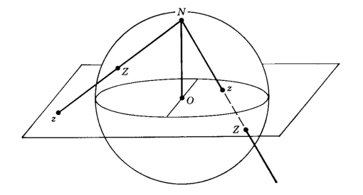
So we have some \(c = \frac{\beta}{\alpha}\). Suppose \(c \neq \infty\). Then this is just a point on the complex plane: \(c = x + iy\). Now imagine there’s a unit sphere at the origin cut at the equator by the complex plane. And imagine you’re standing at the South Pole, and you have a laser pointer, and you point the beam at \(c\).
The beam will intersect the sphere in exactly one location. If \(c\) is outside the unit circle on the plane, you’ll get a point on the southern hemisphere, and if \(c\) is inside the unit circle, you’ll get a point on the northern hemisphere. Every point in the plane, in this way, can be mapped to a point on the sphere–except we have a point left over, the South Pole itself! So if \(\alpha = 0\), and therefore \(c = \infty\), we map that point to the South Pole. In other words, we can think of \(z = \frac{\beta}{\alpha}\) as being a point on the extended complex plane (the plane plus an extra point at infinity), which is just the sphere. This map is known as the stereographic projection.
Explicitly, if \(c = x + iy\), then we have \((\frac{2x}{1+x^2+y^2}, \frac{2y}{1+x^2+y^2}, \frac{1-x^2-y^2}{1+x^2+y^2})\) or \((0,0,-1)\) if \(z=\infty\).
Below, the map is depicted (where the pole of projection is the North Pole):

Moreover, we can go in reverse: \(c = \frac{x}{1+z} + i\frac{y}{1+z}\) or \(\infty\) if \(z=-1\).
[19]:
c = spinor_c(qubit) # gives us our complex ratio
print("c: %s" % c)
xyz = c_xyz(c) # stereographically projects to the sphere
print("xyz: %s" % xyz)
c: (-0.9905580099071644-0.08527276925028497j)
xyz: [-0.99629837 -0.08576693 0.00579508]
As you can see, we get the same point which we obtained before via the expectation values \((\langle \hat{X} \rangle, \langle \hat{Y} \rangle, \langle \hat{Z} \rangle)\). Moreover, it’s clear that every state will give us a unique point on the sphere, and vice versa, up to complex phase. And the bit about the phase is true because clearly if we rephase both \(\alpha\) and \(\beta\) by the same amount in \(c = \frac{\beta}{\alpha}\), we’ll end up with the same \(c\). And we’re only allowed to rephase, and not rescale, because of the normalization condition \(|\alpha|^2 + |\beta|^2 = 1\).
And by the way, the phase matters: watch what happens to the phase (depicted in green), as we do a full rotation:
[ ]:
scene = vp.canvas(background=vp.color.white)
m = MajoranaSphere(qubit, show_phase=True, scene=scene)
m.snapshot()
m.evolve(qt.jmat(1/2, 'y'), T=2*np.pi)
The phase goes to the negative of itself. Only after a full two turns does the state come back to itself completely, and this is what characterizes spin-\(\frac{1}{2}\) representations. \(SU(2)\) is the double cover of \(SO(3)\) and what this means is that for every element in the usual rotation group, there are two elements of \(SU(2)\).
[ ]:
scene = vp.canvas(background=vp.color.white)
m = MajoranaSphere(qubit, show_phase=True, scene=scene)
m.snapshot()
m.evolve(qt.jmat(1/2, 'y'), T=4*np.pi)
In any case, by means of the stereographic projection, we obtain the “Riemann sphere” (here depicted with the North Pole being the pole of projection:

We’ve just seen how each these cardinal directions can be associated with qubit states: in fact, the eigenstates of the Pauli matrices. And thus we observe the interesting fact that antipodal points on the sphere become orthogonal vectors in Hilbert space.
[20]:
print([spinor_c(v) for v in qt.sigmax().eigenstates()[1]])
print([spinor_c(v) for v in qt.sigmay().eigenstates()[1]])
print([spinor_c(v) for v in qt.sigmaz().eigenstates()[1]])
[(-1+0j), (1.0000000000000002+0j)]
[-1j, (-0+1.0000000000000002j)]
[inf, 0j]
spheres.coordinates provides useful functions for going back and forth between coordinate systems on the sphere. E.g.:
[21]:
print(xyz_c(xyz)) # back to extended complex coordinates
print(xyz_sph(xyz)) # spherical coordinates
print(c_sph(c)) # spherical coordinates, etc
print(c_spinor(c)) # back to a qubit, up to phase
print(compare_nophase(qubit, c_spinor(c)))
(-0.9905580099071642-0.08527276925028496j)
[1.56500121 3.22746653]
[1.56500121 3.22746653]
Quantum object: dims = [[2], [1]], shape = (2, 1), type = ket
Qobj data =
[[ 0.70915269+0.j ]
[-0.70245688-0.06047141j]]
True
A “constellation”
So we can represent a spin-\(\frac{1}{2}\) state by a point on the “Bloch sphere” plus a complex phase, which gives us an intuitive geometrical picture of the quantum state, one which isn’t immediately obvious when you look at it represented as a complex linear superpositon, say, of \(Z\) eigenstates.
But what about higher spin states? Recall that spin representations are labeled by \(j\) values, which count up from \(0\) by half integers, and their dimensionality is \(2j + 1\). Each basis state is associated with an \(m\) value ranging from \(-j\) to \(j\), counting up by \(1\). So basis states can be labeled \(\mid j, m \rangle\). E.g.:
For spin-\(0\): \(\mid 0, 0 \rangle\).
For spin-\(\frac{1}{2}\): \(\mid \frac{1}{2}, \frac{1}{2} \rangle, \mid \frac{1}{2}, -\frac{1}{2} \rangle\).
For spin-\(1\): \(\mid 1, 1 \rangle, \mid 1, 0 \rangle, \mid 1, -1 \rangle\).
For spin-\(\frac{3}{2}\): \(\mid \frac{3}{2}, \frac{3}{2} \rangle, \mid \frac{3}{2}, \frac{1}{2} \rangle, \mid \frac{3}{2}, -\frac{1}{2} \rangle, \mid \frac{3}{2}, -\frac{3}{2} \rangle\).
And so on.
One might wonder if our simple geometrical representation for a qubit generalizes for higher spin. And the answer is yes! In fact, it was first proposed way back in 1932 by Ettore Majorana. The answer is both simple and elegant: a spin-\(j\) state can be represented by a constellation of \(2j\) points on the sphere (up to phase). These points are often poetically termed “stars” in the literature.
So just as a spin-\(\frac{1}{2}\) can be specified by a point on a sphere, a spin-\(1\) state can be specified by two points on the sphere, a spin-\(\frac{3}{2}\) state by three points on the sphere, and so on (again, up to phase).

The basic construction is this.
Given a spin-\(j\) state in the \(\mid j, m \rangle\) representation, \(\mid \psi \rangle = \begin{pmatrix}a_{0} \\ a_{1} \\ a_{2} \\a_{3} \\ \vdots\end{pmatrix}\), form a complex polynomial in an unknown \(z\):
The roots of this polynomial, called the Majorana polynomial, when stereographically projected from the complex plane to the sphere, yield the constellation. If you lose a degree, (i.e. if the coefficients for the highest powers of \(z\) are \(0\)) then you add a root “at infinity” for each one, and so the spin-\(j\) state can always be specified by \(2j\) point on the sphere.
In other words, by the fundamental theorem of algebra, no less, a spin-\(j\) state factorizes into \(2j\) pieces.

As the above image indicates, the \(\mid j, m\rangle\) basis states (assuming we’ve quantized along the \(Z\) direction) consist of (in the case of spin-\(\frac{3}{2}\)) three stars at the North Pole, none at the South Pole; two stars at the North Pole, one at the South Pole; one at the North Pole, two at the South Pole; none at the North Pole, three at the South Pole. Any spin state can be expressed as a complex linear superposition of these basis states/constellations.
At the same time, thanks to Majorana, we can also interpret the spin state as a polynomial and find its roots. Each corresponds to a little monomial whose product (as opposed to sum) determines the same state. Each root is associated with a direction in 3D, and under rotations, the stars transform rigidly as a whole constellation.
[22]:
from spheres import *
spin = xyz_spin([[1,0,0], [0,1,0],[0,0,1]])
print("cartesian stars:\n%s" % spin_xyz(spin))
print("spherical stars:\n%s" % spin_sph(spin))
print("extended complex stars:\n%s" % "\n".join([str(c) for c in spin_c(spin)]))
cartesian stars:
[[2.22044605e-16 1.00000000e+00 2.22044605e-16]
[1.00000000e+00 8.32667268e-17 2.22044605e-16]
[0.00000000e+00 0.00000000e+00 1.00000000e+00]]
spherical stars:
[[1.57079633e+00 1.57079633e+00]
[1.57079633e+00 8.32667268e-17]
[0.00000000e+00 0.00000000e+00]]
extended complex stars:
(2.220446049250313e-16+0.9999999999999998j)
(0.9999999999999998+8.326672684688674e-17j)
0j
[ ]:
scene = vp.canvas(background=vp.color.white)
m = MajoranaSphere(spin, scene=scene)
m.evolve(qt.jmat(3/2, 'y'), dt=0.01, T=5)
We can use matplotlib for this too:
[23]:
%matplotlib notebook
anim = animate_spin(spin, qt.jmat(3/2, 'y'))

We can understand the Majorana polynomial a little better by considering Vieta’s formulas which relate the roots to the coefficients of a polynomial.
Given a polynomial \(f(z) = c_{n}z^n + c_{n-1}z^{n-1} + \dots + c_{1}z + c_{0}\), if we denote its roots by \(r_{i}\), we can write:
\(c_{n} = c_{n}\)
\(c_{n-1} = -c_{n}\big{[} r_{1} + r_{2} + \dots \big{]}\)
\(c_{n-2} = c_{n}\big{[} r_{1}r_{2} + r_{1}r_{3} + r_{2}r_{3} + \dots \big{]}\)
\(c_{n-3} = -c_{n}\big{[} r_{1}r_{2}r_{3} + r_{1}r_{2}r_{4} + r_{2}r_{3}r_{4} + \dots \big{]}\)
\(\vdots\)
\(c_{0} = (-1)^{n} c_{n} \big{[} r_{1}r_{2}\dots r_{n} \big{]}\)
In other words, if we divide out by the leading coefficient \(c_{n}\), which doesn’t affect the roots, the \(c_{0}\) coefficient is given \((-1)^n\) times the product of the roots, the \(c_{1}\) coefficient is given by \((-1)^{n-1}\) times the sum of the products of pairs of roots, the \(c_{2}\) coefficient is given by \((-1)^{n-2}\) times the sum of products of triples of roots, and so forth. In each of these expressions, there will be \(\binom{n}{n-k}\) terms corresponding to \(c_{k}\).
So reading the Majorana formula in reverse, it tells us that if we want to go from a polynomial to a spin state, we should divide each coefficient by the square root of the number of terms in Vieta’s formula that contribute to it, and multiply by the power of \(-1\).
The importance of the latter becomes clear, if we consider the simplest case of a monomial (aka a qubit). Suppose we want the star to be in the \(X+\) direction. As an unnormalized spin state, this is \(\begin{pmatrix} 1 \\ 1 \end{pmatrix}\), and as an extended complex coordinate, this is just \(z=1\). So our monomial is \(z - 1 = 0\). But if we want to convert the coefficients of this monomial into the components of the spin, we have to flip the negative sign. The powers of \(-1\) in the Majorana formula handle this in the general case.
Here are some interesting videos showing the dynamics. As I said, a rotation rotates all the stars individually:

If a spin is in an eigenstate of some Hamiltonian, its constellation will be fixed. But if you perturb it out of the eigenstate, the stars will precess around their former locations:

This can lead to some cool effects:

If you perturb them far enough, they start to swap places:

And finally, you can have as many stars as you please! They look like little charged particle confined to the surface of the sphere, and there is indeed something to that analogy as work by Leboeuf and Bruno have shown.

Check out the documentation for MajoranaSphere to learn how to leave trails (set make_trails=True), as well as how to set the color of the stars. Beware though, if you do this, there may be some numerical errors, since when the polynomial solver returns the roots, they won’t necessarily be in the same order every time! I have a hack to get around this, but it isn’t perfect.
Spin Coherent States
Probably the best way to understand why the Majorana construction works is in terms of “spin coherent states.” Spin coherent states have all their angular momentum concentrated in one direction on the sphere. In other words, all their “stars” all coincide at just one point. As such, for a given \(j\) value, there is a spin coherent state for each point on the sphere. It turns out that the spin coherent basis form an overcomplete basis or “frame” for spin states. This is, of course, not an othogonal basis, and indeed, there are an infinite number of elements: but knowing the amplitudes of a given spin state on each of the spin coherent states determines the state. In other words, the spin coherent states form a resolution of the identity.
So for example, just as we write \(\psi(x)\) for \(\langle x \mid \psi \rangle\) for a position wavefunction, for a spin, we could write \(\psi(\tilde{z}) = \langle \tilde{z} \mid \psi \rangle\), where \(\tilde{z}\) represents a point on the sphere given as a extended complex coordinate.
Now it turns out, if we normalize our Majorana polynomial \(p(z)\) from before:
\(p(z) = \frac{e^{-2ij\theta}}{(1+r^2)^j} \sum_{m=-j}^{m=j} (-1)^{j+m} \sqrt{\binom{2j}{j-m}} a_{j+m} z^{j-m}\)
Where \(z=re^{i\theta}\), then:
\(\langle \tilde{z} \mid \psi \rangle = p(z)\)
Where \(\tilde{z}\) is the point antipodal to \(z\) on the sphere, and \(\mid \tilde{z} \rangle\) is the spin coherent state with all the stars at the point \(\tilde{z}\). Note that to evaluate the Majorana polynomial at \(\infty\), it suffices to return the coefficient corresponding to the highest degree (and normalized in the above case). This amounts to evaluating the polynomial at 0 in a flipped coordinate chart.
In other words, the spin coherent amplitude will always be 0 opposite to a Majorana star. Another way of saying this is that the Majorana stars represent those directions for which there is a 0% chance that all the angular momentum will be concentrated in the opposite direction. This gives them an operational meaning: if I send a spin through a Stern-Gerlach oriented in the direction of a star, then there’s a 0% chance that it’ll be found in the state with all the angular momentum in the opposite direction. Moreover, the spin state is fully characterized by these 0 probability points. Indeed, one can work with the probability distribution itself (often called a Husimi distribution) with no loss of generality (up to phase), since it has the same 0’s.
Note that the normalization makes the resulting function non-holomorphic.
[29]:
from spheres import *
j = 3/2
spin = qt.rand_ket(int(2*j+1))
p = spin_poly(spin, projective=True, normalized=True)
s = lambda z: (spin_coherent(j, antipodal(z), from_complex=True).dag()*spin)[0][0][0]
c = rand_c()
print("majorana: %s" % p(c))
print("spin coherent: %s" % s(c))
majorana: (0.5726321887977408+0.36878212146672185j)
spin coherent: (0.5726321887977408+0.3687821214667217j)
We could have also done it in terms of cartesian coordinates:
[30]:
from spheres import *
j = 3/2
spin = qt.rand_ket(int(2*j+1))
p = spin_poly(spin, cartesian=True, normalized=True)
s = lambda xyz: (spin_coherent(j, -xyz).dag()*spin)[0][0][0]
xyz = rand_xyz()
print("majorana: %s" % p(xyz))
print("spin coherent: %s" % s(xyz))
majorana: (-0.3381956446920869-0.3644345696570041j)
spin coherent: (-0.33819564469208685-0.3644345696570041j)
If we further normalize the Majorana polynomial by \(\sqrt{\frac{2j+1}{4\pi}}\), then we can express the inner product between two spin states as an integral over the sphere:
[31]:
from spheres import *
a = qt.rand_ket(3)
b = qt.rand_ket(3)
print("amplitude: %s " % (a.dag()*b)[0][0][0])
a_func = spin_poly(a, for_integration=True)
b_func = spin_poly(b, for_integration=True)
import quadpy
scheme = quadpy.u3.get_good_scheme(19)
print("amplitude %s" % scheme.integrate_spherical(lambda sph: a_func(sph).conj()*b_func(sph)))
print("amplitude %s" % spherical_inner(a_func, b_func))
amplitude: (0.15085036103837118+0.6265137597537351j)
amplitude (0.15085036103837118+0.6265137597537351j)
amplitude (0.15085036103837118+0.6265137597537351j)
We can visualize the spin coherent amplitudes as arrows at each point on the sphere. Observe how the “spin coherent wavefunction” is 0 opposite to the stars.
[ ]:
from spheres import *
scene = vp.canvas(background=vp.color.white)
spin = qt.rand_ket(3)
m = MajoranaSphere(spin, show_wavefunction=True, wavefunction_type="coherent", scene=scene)
Alternatively, we can visualize the normalized Majorana function itself whose 0’s are the stars.
[ ]:
scene = vp.canvas(background=vp.color.white)
n = MajoranaSphere(spin, show_wavefunction=True, wavefunction_type="majorana", scene=scene)
Finally, here’s a cute algebraic demonstration of why this works:
Suppose we have some spin-\(1\) vector: \(\mid \psi \rangle = \begin{pmatrix} a \\ b \\ c \end{pmatrix}\). Its Majorana polynomial is \(p(z) = az^2 - \sqrt{2}bz + c\).
Meanwhile, we form a spin-\(1\) coherent polynomial, which will have two stars at a given point \(\alpha\):
\((z - \alpha)^{2} = z^{2} - 2\alpha z + \alpha^2\)
And then convert it into a ket: \(\begin{pmatrix} 1 \\ \frac{2}{\sqrt{2}}\alpha \\ \alpha^{2} \end{pmatrix}\) = \(\begin{pmatrix} 1 \\ \sqrt{2} \alpha \\ \alpha^{2} \end{pmatrix}\) .
Now let’s rename \(\alpha\) to \(z\): \(\begin{pmatrix} 1 \\ \sqrt{2} z \\ z^{2} \end{pmatrix}\)
Just for show, why not normalize it?
\(N = \frac{1}{\sqrt{1 + 2zz^{*} + (z^2)(z^2)^{*}}} = \frac{1}{\sqrt{1 + 2|z|^2 + |z|^4}} = \frac{1}{\sqrt{(1 + |z|^2)^{2}}} = \frac{1}{1 + |z|^2}\)
Giving: \(\frac{1}{1 + |z|^2} \begin{pmatrix} 1 \\ \sqrt{2}z \\ z^{2} \end{pmatrix}\).
Now let’s form the inner product \(\langle \psi \mid z \rangle\). (Technically, we want \(\langle z \mid \psi \rangle\), but \(\langle z \mid \psi \rangle = \langle \psi \mid z \rangle^{*}\), and this is easier for this demonstration.)
\(\begin{pmatrix} a^{*} & b^{*} & c^{*} \end{pmatrix} \frac{1}{1 + |z|^2} \begin{pmatrix} 1 \\ \sqrt{2}z \\ z^{2} \end{pmatrix} = \frac{1}{1 + |z|^2} \big{(} a^{*} + \sqrt{2}b^{*}z + c^{*}z^{2} \big{)}\)
So now we have: \(h(z) = \frac{1}{1 + |z|^2} \big{(} c^{*}z^{2} + \sqrt{2}b^{*}z + a^{*} \big{)}\).
Now it happens that if we take a complex vector, flip its components left/right, complex conjugate the elements, and flip every other sign, then we get the antipodal constellation.
[32]:
spin = qt.rand_ket(5)
print("stars:\n%s" % spin_xyz(spin))
antipodal_spin = qt.Qobj(np.array([c*(-1)**i for i, c in enumerate(components(spin).conj()[::-1])]))
print("antipodal stars:\n%s" % spin_xyz(antipodal_spin))
stars:
[[ 0.61569799 -0.18244856 -0.76656931]
[ 0.81965758 -0.55147919 0.15502305]
[-0.08533574 0.98796788 0.12898561]
[-0.98417313 0.11334806 0.13621846]]
antipodal stars:
[[ 0.98417313 -0.11334806 -0.13621846]
[ 0.08533574 -0.98796788 -0.12898561]
[-0.81965758 0.55147919 -0.15502305]
[-0.61569799 0.18244856 0.76656931]]
So let’s do that:
So: \(h(z) \rightarrow p(z) = \frac{1}{1 + |z|^2} \big{(} az^{2} - \sqrt{2}bz + c \big{)}\).
Ignoring the normalization, which was just for fun, and plugging this into the reverse Majorana polynomial, we obtain the ket: \(\begin{pmatrix} a \\ b \\ c \end{pmatrix}\), which is exactly what we started with.
Bibliography
Geometry of quantum states : an introduction to quantum entanglement
Coherent-State Approach for Majorana Representation
Phase space approach to quantum dynamics
Majorana Representation of Higher Spin States
Quantum Geometric Phase in Majorana’s Stellar Representation: Mapping onto a Many-Body Aharonov-Bohm
How to Prepare a Permutation Symmetric Multiqubit State on an Actual Quantum Computer
It turns out that one can represent a spin-\(j\) state equivalently as a permutation symmetric state of \(2j\) qubits. And this is good because given that our quantum computers (mostly) work with qubits, we need a way to represent everything we might care about in terms of them.
For example, if we have a spin-\(\frac{3}{2}\) state, we could express it in the usual \(\mid j, m \rangle\) basis as:
or in terms of symmeterized qubits:
In other words, there’s a one-to-one correspondence between the four \(\mid j, m \rangle\) basis states and the four symmetric basis states of three qubits. To wit: the states with \(3 \uparrow\), with \(2 \uparrow, 1 \downarrow\), with \(2 \downarrow, 1 \uparrow\), and with \(3 \downarrow\).
So we can easily form a linear map that takes us from the one representation to the other:
[1]:
from spheres import *
def symmetrize(pieces):
return sum([qt.tensor(*[pieces[i] for i in perm]) for perm in permutations(range(len(pieces)))]).unit()
def spin_sym_map(j):
if j == 0:
return qt.Qobj(1)
S = qt.Qobj(np.vstack([\
components(symmetrize(\
[qt.basis(2,0)]*int(2*j-i)+\
[qt.basis(2,1)]*i))\
for i in range(int(2*j+1))]).T)
S.dims =[[2]*int(2*j), [int(2*j+1)]]
return S
j = 3/2
d = int(2*j+1)
S = spin_sym_map(j)
spin = qt.rand_ket(d)
sym = S*spin
print("spin state:\n%s" % spin)
print("\npermutation symmetric qubits:\n%s" % sym)
I = S.dag()*S
print("\ntransformation an isometry?: %s" % (I == qt.identity(I.shape[0])))
spin state:
Quantum object: dims = [[4], [1]], shape = (4, 1), type = ket
Qobj data =
[[ 0.2680114 -0.33141963j]
[-0.06116115+0.26914443j]
[-0.54797038-0.31029464j]
[-0.58359679-0.07079553j]]
permutation symmetric qubits:
Quantum object: dims = [[2, 2, 2], [1]], shape = (8, 1), type = ket
Qobj data =
[[ 0.2680114 -0.33141963j]
[-0.0353114 +0.15539061j]
[-0.0353114 +0.15539061j]
[-0.31637084-0.17914869j]
[-0.0353114 +0.15539061j]
[-0.31637084-0.17914869j]
[-0.31637084-0.17914869j]
[-0.58359679-0.07079553j]]
transformation an isometry?: True
Another way of obtaining the same result is to find the roots of the Majorana polynomial of the spin, map the complex roots to the sphere, convert each resulting point into a qubit, and then symmeterize those separable qubits. Well, technically, if we do this, we lose the overall phase information of the original spin, but such is life.
Just for reference, again here’s the Majorana polynomial:
Where the \(a\)’s run through the components of the spin. Recall that if we have an \(d\) dimensional spin vector, but end up with a less than \(d\) degree polynomial, we add a root at infinity for each missing degree. Having obtained the roots, we stereographically project them to the sphere to get \((x, y, z)\) points, which we enjoy poetically calling “stars.”
The connection to permutation symmetry is that the roots are contained “unordered” in the polynomial!
Below we take a spin, finds its stars, convert them into qubits, symmeterize the qubits, then use the inverse of the transformation above to get back the spin state, and find the stars again. We see we recover the original stars exactly. So we get the right result up to phase. (Note we could have converted the complex roots directly to qubits, as we’ve seen, insofar as each complex root is to be the ratio between the two components of the qubit.)
[4]:
stars = spin_xyz(spin)
qubits = [qt.Qobj(xyz_spinor(star)) for star in stars]
sym2 = symmetrize(qubits)
spin2 = S.dag()*sym2
stars2 = spin_xyz(spin2)
print("initial stars:\n%s\n" % "\n".join([str(star) for star in stars]))
print("final stars:\n%s\n" % "\n".join([str(star) for star in stars2]))
initial stars:
[-0.74108075 -0.2676052 -0.61578144]
[ 0.32802509 0.85798535 -0.39529822]
[ 0.63479369 -0.38107314 0.67217574]
final stars:
[-0.74108075 -0.2676052 -0.61578144]
[ 0.32802509 0.85798535 -0.39529822]
[ 0.63479369 -0.38107314 0.67217574]
Another way of saying this is that if we have a state of \(2j\) separable qubits, each with an \((x, y, z)\) point representing its expected rotation axis, if we permute the qubits in all possible orders and add up all these permuted states, then the resulting state is naturally permutation symmetric, but also perhaps remarkably preserves the \((x, y, z)\) points of each of the qubits. Each point is now encoded not individually in the separable qubits, but instead holistically in the state of the entangled whole. If we transform from the symmeterized qubits to a spin-\(j\) state and find the roots of the Majorana polynomial, these complex roots, stereographically projected to the sphere, gives us back our original \((x, y, z)\) points. Of course, we have thrown out some information: namely, the phases of the individual qubits we symmeterized.
That’s all well and good, but a moment’s reflection will convince you that the operation of symmeterizing a bunch of qubits is not a unitary operation. After all, I need to make a separate copy of the qubits, one for each possible permutation, and then add them all up. This of course would violate no-cloning.
So you might wonder: Suppose I have \(2j\) separable qubits loaded into my quantum computer, and I want to prepare the permutation symmetric state corresponding to them. How do I do it?! Clearly, there can be no deterministic quantum operation that will do the trick.
Well, in this game, what one can’t do deterministically, one can often do probablistically. And that turns out to be the case here.
Consider the following circuit:

The heart of this circuit is the “controlled swap” or Fredkin gate. This is a three qubit gate: if the first qubit is \(\uparrow\), it leaves the second two alone; but if the first qubit is \(\downarrow\), it swaps/permutes the second two.
Its matrix representation is:
Which is easily obtained insofar as its just a \(4 \times 4\) identity block concatenated with the usual swap gate:
By the way, that’s a general rule for constructing controlled gates: just take the gate you want to be controlled by the first qubit, and concatenate it with an identity matrix of the same dimensionality.
So we have our two qubits we want to symmetrize, and the control qubit, with starts in the \(\mid \uparrow \rangle\) state. We apply a Hadamard gate to the control, which takes it to an even superposition \(\frac{1}{\sqrt{2}}(\mid \uparrow \rangle + \mid \downarrow \rangle\). So then when we apply the Fredkin, the two qubits to be symmetrized end up in a superposition of being swapped and not being swapped, relative to the control. We then apply a Hadamard again to the control, which by the way, is its own inverse (\(H = H^{\dagger}\)), to undo that original rotation, while leaving it entangled with the two qubits.
We then measure the control qubit: if we get \(\uparrow\), then our two qubits \(\mid \psi \rangle\) and \(\mid \phi \rangle\) end up in the symmetrized state \(\frac{1}{\sqrt{2}}(\mid \psi \rangle\mid \phi \rangle + \mid \phi \rangle\mid \psi \rangle)\). On the other hand, we get \(\downarrow\), then our two qubits ends up in the antisymmetrized state: \(\frac{1}{\sqrt{2}}(\mid \psi \rangle\mid \phi \rangle - \mid \phi \rangle\mid \psi \rangle)\).
So if we want the symmetrized state, we just keep doing the experiment over and over again until we get the answer we want!
In the diagram above, you may note there are also two phase rotation gates. We can use those if we want a state of the form \(\frac{1}{\sqrt{2}}(\mid \phi \rangle \mid \psi \rangle + e^{i\theta}\mid \psi \rangle \mid \phi \rangle\). If \(\theta=0\), we just get the identity matrix for both of them, and everything is as I said above.
[5]:
from scipy.linalg import block_diag
# construct our operators
H = (1/np.sqrt(2))*qt.Qobj(np.array([[1,1],\
[1,-1]]))
SWAP = qt.Qobj(np.array([[1,0,0,0],\
[0,0,1,0],\
[0,1,0,0],\
[0,0,0,1]]))
CSWAP = qt.Qobj(block_diag(np.eye(4), SWAP.full()))
CSWAP.dims = [[2,2,2], [2,2,2]]
theta = 0
P1 = qt.Qobj(np.array([[np.exp(1j*theta/2), 0],\
[0, 1]]))
P2 = qt.Qobj(np.array([[1, 0],\
[0, np.exp(1j*theta/2)]]))
CIRCUIT = qt.tensor(H, qt.identity(2), qt.identity(2))*\
qt.tensor(P2, qt.identity(2), qt.identity(2))*\
CSWAP*\
qt.tensor(P1, qt.identity(2), qt.identity(2))*\
qt.tensor(H, qt.identity(2), qt.identity(2))
c = qt.basis(2,0) # control
a, b = qt.rand_ket(2), qt.rand_ket(2) # to be symmetrized
state = qt.tensor(c, a, b)
def measure_control(state):
Zl, Zv = qt.sigmaz().eigenstates()
Zp = [v*v.dag() for v in Zv][::-1]
dm = state.ptrace(0).full().real
which = np.random.choice(list(range(2)), p=np.diag(dm))
print("p(up): %.4f" % (dm[0,0]))
print("p(down): %.4f" % (dm[1,1]))
print("obtained: %s" % ("up" if which == 0 else "down"))
return which, (qt.tensor(Zp[which], qt.identity(2), qt.identity(2))*state).unit()
which, state = measure_control(CIRCUIT*state)
answer = state.ptrace((1,2)) # throw out the control
correct_sym = (qt.tensor(a,b) + qt.tensor(b,a)).unit()
correct_sym = correct_sym*correct_sym.dag()
correct_antisym = (qt.tensor(a,b) - qt.tensor(b,a)).unit()
correct_antisym = correct_antisym*correct_antisym.dag()
if which == 0:
print("got correct symmetrized state?: %s" % (answer == correct_sym))
else:
print("got correct antisymmetrized state?: %s" % (answer == correct_antisym))
p(up): 0.6648
p(down): 0.3352
obtained: up
got correct symmetrized state?: True
Okay, so that’s great, but what if we have multiple qubits we want to symmetrize?
The simplest thing to do is a direct generalization of the above. If we have \(n\) qubits, there will be \(n!\) possible permutations. So we’ll need a control qudit that lives in \(n!\) dimensions. For example, for \(3\) qubits, there are \(3! = 6\) possible permutations, so we need a control state that is \(6\) dimensional. We start with the control in its \(\mid 0 \rangle\) state, and the apply the Hadamard in \(n!\) dimensions, in other words, the Quantum Fourier Transform, which takes \(\mid 0 \rangle\) to an even superposition of all its basis states. We then do a controlled operation, which makes performing the \(i^{th}\) permutation on the \(n\) qubits depend on the control being in the \(\mid i \rangle\) basis state. So we end up with the \(n\) qubits being in a superposition of being permuted in all possible ways, relative to the control. Then we apply the inverse QFT to the control, and then measure the control: if it ends up back in the \(\mid 0 \rangle\) state, then the \(n\) qubits are in the permutation symmetric state. Sweet!
You might wonder how to contruct such a controlled permutation gate. In braket notation, you can think of it like:
In other words, we sum over all the permutations \(p_{i}\) (where the \(i\) labels both a basis state of the control \(\mid i \rangle\), and also \(P_{i}\), the operator which performs that permutation of the qubits), and also over the \(2^n\) basis states of the \(n\) qubits, labeled by \(j\): \(\mid j \rangle\). Clearly, if this operator acts on a state coming in on the right, it will perform the \(i^{th}\) permutation to the extent that the control is in the \(i^{th}\) state.
Let’s check it out:
[19]:
import math
from itertools import product
# constructs a unitary operation that performs
# the provided permutation of qubit subsystems
def construct_permuter(perm):
indices = [[(i, j) for j in range(2)] for i in range(len(perm))]
tensor_indices = list(product(*indices))
pindices = [[(i, j) for j in range(2)] for i in perm]
ptensor_indices = list(product(*pindices))
m = np.zeros((len(tensor_indices),len(tensor_indices)))
for i, pind in enumerate(ptensor_indices):
m[i, [tensor_indices.index(p) for p in permutations(pind) if p in tensor_indices][0]] = 1
return qt.Qobj(m)
# quantum fourier transform of dimension d
def construct_qft(d):
w = np.exp(2*np.pi*1j/d)
return (1/np.sqrt(d))*\
qt.Qobj(np.array([[w**(i*j)\
for j in range(d)]\
for i in range(d)]))
# constructs a unitary operator that does each of n!
# permutations of n qubits relative to a control of
# dimensionality n!
def construct_cnrl_permutations(n):
d = 2**n
r = math.factorial(n)
perms = list(permutations(list(range(n))))
O = sum([qt.tensor(qt.basis(r, i), construct_permuter(p)*qt.basis(d, j))*\
qt.tensor(qt.basis(r, i), qt.basis(d, j)).dag()\
for j in range(d) for i, p in enumerate(perms)])
O.dims = [[r]+[2]*n, [r]+[2]*n]
return O
################################################################################
n = 3
r = math.factorial(n)
qubits = [qt.rand_ket(2) for i in range(n)]
QFT = qt.tensor(construct_qft(r), *[qt.identity(2)]*n)
CPERMS = construct_cnrl_permutations(n)
PROJ = qt.tensor(qt.basis(r, 0)*qt.basis(r, 0).dag(), *[qt.identity(2)]*n)
state = qt.tensor(qt.basis(r, 0), *qubits)
state = QFT.dag()*CPERMS*QFT*state
# We're lazy, so let's just project into the right state, regardless of probability
final_state = (PROJ*state).unit().ptrace(list(range(1, n+1))) # throw out the control
correct_state = symmetrize(qubits)
correct_state = correct_state*correct_state.dag()
print("got the right permutation symmetric state?: %s" % (final_state == correct_state))
got the right permutation symmetric state?: True
Okay, the final concern you might have is that our control system is \(n!\) dimensions, where \(n\) is the number of qubits we want to symmetrize. We, however, want to formulate everything in terms of qubits. Is there a way of using several qubits as controls to get the same effect? Yes! And here’s how, thanks to Barenco, Berthiaume, Deutsch, Ekert, Jozsa, and Macchiavello (see reference at the end!).
The basic conceptual idea is that permutations can be broken down recursively into a a series of swaps. E.g., suppose we start with an element \(A\). We pop another element \(B\) to the right, and perform the two possible permutations, the identity and the swap:
.
These are the two possible permutations of two elements. We could pop another element \(C\) to the right in each case: \(A \rightarrow AB(C), BA(C)\), and then do all the possible swaps with \(C\):
and
Indeed, these are the six possible permutations of three elements. We could pop another element \(D\) to the right, and do all the possible swaps with \(D\):
These are the 24 possible permutations of four elements, and so on. So what we have to do is translate this idea into a quantum circuit, controlling the individual swaps with qubits.
First off, let’s define:
The point of these guys it to prepare our control qubits. If we have \(k\) control qubits in the \(\mid 0, 0, 0, \dots \rangle\) state, if we apply \(R_{k}\) to the first qubit, and \(T_{k, j}\)’s to adjacent qubits along the line (from \(j=1\) to \(j = k-1\)), then we’ll end up in the state:
In other words, a superposition over all the qubits being \(\uparrow\) or just one of the qubits being \(\downarrow\). (Recall in this notation \(\mid 0 \rangle\) = \(\mid \uparrow \rangle\), etc.) This is the qubit equivalent of our control qudit from before being prepared in an even superposition of all its basis states. Call this whole procedure \(U_{k}\).
So we have \(k\) control qubits prepared. In line with the recursive permutation procedure above, this is in the context of having already symmetrized \(k\) qubits and we want to symmetrize an additional \(k+1^{th}\) qubit. Having prepared the \(k\) control qubits, we apply \(k\) Fredkin gates. If \(j\) runs from \(1\) to \(k\), then the \(j^{th}\) Fredkin uses the \(j^{th}\) control qubit to condition the swapping of the \(j^{th}\) and \(k+1^{th}\) qubits. Then, we as before apply the inverse of the preparation of the control qubits, \(U_{k}^{\dagger}\).
The whole construction is “cascaded” for \(k = 1,2,\dots,n-1\), where \(n\) is the number of qubits we want to symmetrize. So we start with \(k=1\): we’ve “already symmetrized” one qubit and we want to symmetrize the next one, so we introduce \(k=1\) control qubits, preparing them, and then fredkin-ing, and unpreparing. Then we move on to \(k=2\), and we add two more control qubits, prepare them, fredkin, and unprepare, etc. In the end, we’ll need \(\frac{n(n-1)}{2}\) control qubits in total: so if \(n=4\), we have \(\frac{4(4-1)}{2} = 6\) control qubits.
Finally, we measure all the controls, and if they’re all in the \(0/\uparrow\) state, then our qubits will have been symmetrized!
Here’s the circuit for the \(n=4\) case:

The key is that, for example, by the third round, the first three qubits have already been symmetrized, so we only need three controlled swaps to symmetrize them with the fourth.
Let’s check it out! (Note that the indices are offset from the discussion above as we start counting from 0 as opposed to 1.)
[25]:
from qutip.qip.operations import fredkin
def Rk(k):
return (1/np.sqrt(k+1))*qt.Qobj(np.array([[1, -np.sqrt(k)],\
[np.sqrt(k), 1]]))
def Tkj(k, j):
T = (1/np.sqrt(k-j+1))*qt.Qobj(np.array([[np.sqrt(k-j+1), 0, 0, 0],\
[0, 1, np.sqrt(k-j), 0],\
[0, -np.sqrt(k-j), 1, 0],\
[0, 0, 0, np.sqrt(k-j+1)]]))
T.dims = [[2,2], [2,2]]
return T
################################################################################
n = 4
r = int(n*(n-1)/2)
qubits = [qt.rand_ket(2) for i in range(n)]
state = qt.tensor(*[qt.basis(2,0)]*r, *qubits)
offset = r
for k in range(1, n):
offset = offset-k
U = upgrade(Rk(k), offset, n+r)
for j in range(k-1):
T = qt.tensor(*[qt.identity(2)]*(offset+j), Tkj(k, j+1), *[qt.identity(2)]*(r+n-offset-j-2))
U = T*U
state = U*state
for j in range(k):
state = fredkin(N=n+r, control=offset+j, targets=[r+j, r+k])*state
state = U.dag()*state
print("used %d control qubits for %d qubits to be symmetrized" % (r, n))
# do our projections
for i in range(r):
state = (tensor_upgrade(qt.basis(2,0)*qt.basis(2,0).dag(), i, len(state.dims[0]))*state).unit()
final_state = state.ptrace(list(range(r, r+n)))
correct_state = symmetrize(qubits)
correct_state = correct_state*correct_state.dag()
print("got the right permutation symmetric state?: %s" % (final_state == correct_state))
used 6 control qubits for 4 qubits to be symmetrized
got the right permutation symmetric state?: True
Finally, let’s run it on an actual quantum computer! We’ll be using IBM’s qiskit for the job. If you look at the circuit preparation, you’ll notice many of the indices have been flipped due to their convention of treating the tensor product of \(A\) and \(B\) as \(B \otimes A\). We prepare our qubits, and then use qiskit’s tomography feature to recover the density matrix of the symmetrized qubits, conditioned on the controls all being \(0\). You can also find the code here. Give it a whirl.
[28]:
import numpy as np
import qutip as qt
from copy import deepcopy
from math import factorial
from itertools import product
from qiskit import QuantumCircuit, execute, ClassicalRegister
from qiskit import Aer, IBMQ, transpile
from qiskit.providers.ibmq.managed import IBMQJobManager
from qiskit.quantum_info.operators import Operator
from qiskit.ignis.verification.tomography import state_tomography_circuits, StateTomographyFitter
from spheres import *
############################################################################
# symmetrized tensor product
def symmetrize(pieces):
return sum([qt.tensor(*[pieces[i] for i in perm]) for perm in permutations(range(len(pieces)))]).unit()
# constructs linear map between spin-j states and the states of
# 2j symmetrized qubits
def spin_sym_map(j):
if j == 0:
return qt.Qobj(1)
S = qt.Qobj(np.vstack([\
components(symmetrize(\
[qt.basis(2,0)]*int(2*j-i)+\
[qt.basis(2,1)]*i))\
for i in range(int(2*j+1))]).T)
S.dims =[[2]*int(2*j), [int(2*j+1)]]
return S
############################################################################
# convert back and forth from cartesian to spherical coordinates
def xyz_sph(xyz):
x, y, z = xyz
return np.array([np.arccos(z/np.sqrt(x**2+y**2+z**2)),\
np.mod(np.arctan2(y, x), 2*np.pi)])
def sph_xyz(sph):
theta, phi = sph
return np.array([np.sin(theta)*np.cos(phi),\
np.sin(theta)*np.sin(phi),\
np.cos(theta)])
############################################################################
# operators for preparing the control qubits
def Rk(k):
return Operator((1/np.sqrt(k+1))*\
np.array([[1, -np.sqrt(k)],\
[np.sqrt(k), 1]]))
def Tkj(k, j):
return Operator((1/np.sqrt(k-j+1))*\
np.array([[np.sqrt(k-j+1), 0, 0, 0],\
[0, 1, np.sqrt(k-j), 0],\
[0, -np.sqrt(k-j), 1, 0],\
[0, 0, 0, np.sqrt(k-j+1)]]))
############################################################################
j = 3/2
backend_name = "qasm_simulator"
shots = 10000
#backend_name = "ibmq_qasm_simulator"
#backend_name = "ibmq_16_melbourne"
#backend_name = "ibmq_athens"
#shots = 8192
############################################################################
d = int(2*j+1)
n = int(2*j)
r = int(n*(n-1)/2)
# construct a spin state, get the XYZ locations of the stars
# and convert to spherical coordinates
spin_state = qt.rand_ket(d)
angles = spin_sph(spin_state)
# the first p qubits are the control qubits
# the next n are the qubits to be symmetrized
circ = QuantumCircuit(r+n)
# rotate the n qubits so they're pointing in the
# directions of the stars
for i in range(n):
theta, phi = angles[i]
circ.ry(theta, r+i)
circ.rz(phi, r+i)
# apply the symmetrization algorithm:
# iterate over k, working with k control qubits
# in each round: apply the preparation to the controls
# (the U's and T's), then the fredkins, then the inverse
# of the control preparation.
offset = r
for k in range(1, n):
offset = offset-k
circ.append(Rk(k), [offset])
for i in range(k-1):
circ.append(Tkj(k, i+1), [offset+i+1, offset+i])
for i in range(k-1, -1, -1): # because it's prettier
circ.fredkin(offset+i, r+k, r+i)
for i in range(k-2, -1, -1):
circ.append(Tkj(k, i+1).adjoint(), [offset+i+1, offset+i])
circ.append(Rk(k).adjoint(), [offset])
# let's look at it!
print(circ.draw())
# create a collection of circuits to do tomography
# on just the qubits to be symmetrized
tomog_circs = state_tomography_circuits(circ, list(range(r, r+n)))
# create a copy for later
tomog_circs_sans_aux = deepcopy(tomog_circs)
# add in the measurements of the controls to
# the tomography circuits
ca = ClassicalRegister(r)
for tomog_circ in tomog_circs:
tomog_circ.add_register(ca)
for i in range(r):
tomog_circ.measure(i,ca[i])
# run on the backend
if backend_name == "qasm_simulator":
backend = Aer.get_backend("qasm_simulator")
job = execute(tomog_circs, backend, shots=shots)
raw_results = job.result()
else:
provider = IBMQ.load_account()
job_manager = IBMQJobManager()
backend = provider.get_backend(backend_name)
job = job_manager.run(transpile(tomog_circs, backend=backend),\
backend=backend, name="spin_sym", shots=shots)
raw_results = job.results().combine_results()
# have to hack the results to implement post-selection
# on the controls all being 0's:
new_result = deepcopy(raw_results)
for resultidx, _ in enumerate(raw_results.results):
old_counts = raw_results.get_counts(resultidx)
new_counts = {}
# remove the internal info associated to the control registers
new_result.results[resultidx].header.creg_sizes = [new_result.results[resultidx].header.creg_sizes[0]]
new_result.results[resultidx].header.clbit_labels = new_result.results[resultidx].header.clbit_labels[0:-r]
new_result.results[resultidx].header.memory_slots = n
# go through the results, and only keep the counts associated
# to the desired post-selection of all 0's on the controls
for reg_key in old_counts:
reg_bits = reg_key.split(" ")
if reg_bits[0] == "0"*r:
new_counts[reg_bits[1]] = old_counts[reg_key]
new_result.results[resultidx].data.counts = new_counts
# fit the results (note we use the copy of the tomography circuits
# w/o the measurements of the controls) and obtain a density matrix
tomog_fit = StateTomographyFitter(new_result, tomog_circs_sans_aux)
rho = tomog_fit.fit()
# downsize the density matrix for the 2j symmerized qubits
# to the density matrix of a spin-j system, and compare
# to the density matrix of the spin we started out with via the trace
correct_jrho = spin_state*spin_state.dag()
our_jrho = sym_spin(qt.Qobj(rho, dims=[[2]*n, [2]*n]))
print("overlap between actual and expected: %.4f" % (correct_jrho*our_jrho).tr().real)
┌─────────┐ ┌──────────┐ ┌──────────┐┌─────────┐
q_0: ─┤ unitary ├───┤1 ├───────────────────■─┤1 ├┤ unitary ├
└─────────┘ │ unitary │ │ │ unitary │└─────────┘
q_1: ───────────────┤0 ├────────────────■──┼─┤0 ├───────────
┌─────────┐ └──────────┘ ┌─────────┐ │ │ └──────────┘
q_2: ─┤ unitary ├─────────────────■─┤ unitary ├─┼──┼────────────────────────
┌┴─────────┴─┐┌────────────┐ │ └─────────┘ │ │
q_3: ┤ RY(1.9336) ├┤ RZ(0.9955) ├─X─────────────┼──X────────────────────────
├────────────┤├────────────┤ │ │ │
q_4: ┤ RY(2.0132) ├┤ RZ(4.5901) ├─X─────────────X──┼────────────────────────
├────────────┤├────────────┤ │ │
q_5: ┤ RY(1.2433) ├┤ RZ(2.9784) ├───────────────X──X────────────────────────
└────────────┘└────────────┘
overlap between actual and expected: 0.9918
One can use spheres.spin_circuits.qiskit to generate such circuits automatically!
Use spin_sym_qiskit(spin) to generate a Qiskit circuit preparing a given spin state (along with some useful information packaged into a dictionary).
Use postselect_results_qiskit(circ_info, raw_results) to do postselection, once you have results.
And finally, use spin_tomography_qiskit(circ_info, backend_name="qasm_simulator", shots=8000) to run the tomography on a desired backend.
[30]:
from spheres import *
spin = qt.rand_ket(3)
correct_dm = spin*spin.dag()
circ_info = spin_sym_qiskit(spin)
tomog_dm = spin_tomography_qiskit(circ_info)
print("overlap between actual and expected: %.4f" % (correct_dm*tomog_dm).tr().real)
overlap between actual and expected: 0.9999
How To Prepare a Spin-j State on a Photonic Quantum Computer
By now we all know and love how a spin-j state can be decomposed into 2j “stars” on the sphere. We’ve used this decomposition to prepare spin-j states in the form of 2j permutation symmetric qubits on IBM’s quantum computer. Here we’ll see how we can use the same decomposition to prepare a spin-j state on a photonic quantum computer, in terms of oscillator modes.
For this, we’ll need to recall the “Schwinger oscillator” formulation of spin, which can be thought of as the second quantization of a qubit. We introduce two harmonic oscillators for each basis state of a qubit (the fundamental, spin-\(\frac{1}{2}\) representation). This actually gives us all the higher spin representations for free. You can think of it like one oscillator counts the number of “\(\uparrow\)” quanta and one oscillator counts the number of “\(\downarrow\)” quanta. The resulting Fock space can be interpreted as describing a theory of a variable number of bosonic spin-\(\frac{1}{2}\) quanta (aka a theory of symmetric multiqubit states with different numbers of qubits), or more simply as a tower of spin states, one for each \(j\).
The easiest way to see this is to rearrange the Fock space of the two oscillators in the follow perspicacious form:
\(\{\mid 00 \rangle, \mid 10 \rangle, \mid 01 \rangle, \mid 20 \rangle, \mid 11 \rangle, \mid 02 \rangle, \mid 30 \rangle, \mid 21 \rangle, \mid 12 \rangle, \mid 03 \rangle, \dots \}\)
In other words, we can consider the subspaces with a fixed total number of quanta:
\(\{ \mid 00 \rangle \}\)
\(\{ \mid 10 \rangle, \mid 01 \rangle \}\)
\(\{ \mid 20 \rangle, \mid 11 \rangle, \mid 02 \rangle \}\)
\(\{ \mid 30 \rangle, \mid 21 \rangle, \mid 12 \rangle, \mid 03 \rangle \}\)
The first subspace is 1 dimensional, and corresponds to a spin-\(0\) state. The second subspace is 2 dimensional, and corresponds to a spin-\(\frac{1}{2}\) state. The third subspace is 3 dimensional, and corresponds to a spin-\(1\) state. The fourth subspace is 4 dimensional, and corresponds to a spin-\(\frac{3}{2}\) state. And so on.
In other words, say, for spin-\(\frac{3}{2}\), we have the correspondence:
\(\mid \frac{3}{2}, \frac{3}{2} \rangle \rightarrow \mid 30 \rangle\)
\(\mid \frac{3}{2}, \frac{1}{2} \rangle \rightarrow \mid 21 \rangle\)
\(\mid \frac{3}{2}, -\frac{1}{2} \rangle \rightarrow \mid 12 \rangle\)
\(\mid \frac{3}{2}, -\frac{3}{2} \rangle \rightarrow \mid 03 \rangle\)
And indeed, if we visualize these basis states, they correspond to: 3 stars at the North Pole; 2 stars at the North Pole, 1 star at the South Pole; 1 star at the North Pole, 2 stars at the South Pole; and 3 stars at the South Pole.
For comparison, here’s the same correspondence in terms of symmetric multiqubit states:
\(\mid \frac{3}{2}, \frac{3}{2}\rangle \rightarrow \ \mid \uparrow \uparrow \uparrow\rangle\)
\(\mid \frac{3}{2}, \frac{1}{2}\rangle \rightarrow \frac{1}{\sqrt{3}} \Big{(} \mid \uparrow \uparrow \downarrow\rangle + \mid \uparrow \downarrow \uparrow \rangle + \mid \downarrow \uparrow \uparrow \rangle \Big{)}\)
\(\mid \frac{3}{2}, -\frac{1}{2}\rangle \rightarrow \frac{1}{\sqrt{3}} \Big{(} \mid \downarrow \downarrow \uparrow \rangle + \mid \downarrow \uparrow \downarrow \rangle + \mid \uparrow \downarrow \downarrow \rangle \Big{)}\)
\(\mid \frac{3}{2}, -\frac{3}{2}\rangle \rightarrow \ \mid \downarrow \downarrow \downarrow \rangle\)
We can see the basis states correspond to a sum over all the states where \(n\) qubits are \(\uparrow\) and \(2j-n\) qubits are down. We can upgrade a spin-j state to the symmetric multiqubit representation by exploiting this correspondence between basis states, or by preparing 2j qubits pointed in the Majorana directions and taking the permutation symmetric tensor product.
The justification for doing this comes from considering the Majorana polynomial.
Given a spin state in the \(\mid j, m \rangle\) representation: $:nbsphinx-math:mid `:nbsphinx-math:psi :nbsphinx-math:rangle `=
$, we form a polynomial in a complex variable \(z\):
\(p(z) = \sum_{m=-j}^{m=j} (-1)^{j+m} \sqrt{\binom{2j}{j-m}} a_{j+m} z^{j-m}\)
Its roots, stereographically projected from the complex plane to the sphere, yield the constellation. And note if you lose a degree, you add a root at “infinity” (conventionally, the South Pole).
In other words:
By the fundamental theorem of algebra, a spin-j state factorizes into 2j pieces: clearly the product of the monomials is independent of the order of multiplication. This corresponds to the permutation symmetric tensor product of qubits, one for each star.
In a second quantization context, we can upgrade a first quantized operator \(\hat{O}\) to a second quantized operator \(\hat{\textbf{O}}\) in an intuitive way:
\(\hat{\textbf{O}} = \sum_{i, j} \hat{a}_{i}^{\dagger}O_{ij}\hat{a}_{j}\)
This can also be interpreting wedging the operator \(\hat{O}\) between a row vector of creation operators and a column vector of annihilation operators.
We can thus construct second quantized representations of the Pauli matrices, which are the generators of \(SU(2)\) rotations. Given two oscillators with annihilation operators \(\hat{a}_{0}\) and \(\hat{a}_{1}\):
\(\hat{\sigma_{X}} \rightarrow \hat{a}_{1}^{\dagger}\hat{a}_{0} + \hat{a}_{0}^{\dagger}\hat{a}_{1}\)
\(\hat{\sigma_{Y}} \rightarrow i(\hat{a}_{1}^{\dagger}\hat{a}_{0} - \hat{a}_{0}^{\dagger}\hat{a}_{1})\)
\(\hat{\sigma_{Z}} \rightarrow \hat{a}_{0}^{\dagger}\hat{a}_{0} - \hat{a}_{1}^{\dagger}\hat{a}_{1}\)
The resulting operators will be block diagonal in terms of the different spin sectors, and perform separate rotations in each sector.
We can also construct creation operators which add a “star.”
Specifically, given a spin-\(\frac{1}{2}\) state \(\begin{pmatrix}\alpha \\ \beta \end{pmatrix}\), we can upgrade it to the operator \(\alpha \hat{a}_{0}^{\dagger} + \beta \hat{a}_{1}^{\dagger}\).
Repeated applications of such star operators allow one to build up a constellation one star at a time. Another way of thinking about this is that we can build an operator which raises an entire constellation in the form of a polynomial in the creation and annihilation operators:
\((\alpha_{0} \hat{a}^{\dagger} + \beta_{0} \hat{b}^{\dagger})(\alpha_{1} \hat{a}^{\dagger} + \beta_{1} \hat{b}^{\dagger})(\alpha_{2} \hat{a}^{\dagger} + \beta_{2} \hat{b}^{\dagger})\dots\)
And this turns out to be the Majorana polynomial in disguise:
\(\sum_{m=-j}^{m=j} \sqrt{\binom{2j}{j-m}} a_{j+m} (\hat{a}^{\dagger})^{j-m}(\hat{b}^{\dagger})^{j+m}\)
Note the \((-1)^{j+m}\) factor dissapears. Why? Consider that if we have \(\alpha z + \beta = z + \frac{\beta}{\alpha} = 0\), we have a root at \(-\frac{\beta}{\alpha}\), and the \((-1)^{j+m}\) corrects for this negative sign. So we need the \((-1)^{j+m}\) when we’re converting from a spin state to a polynomial to get the correct results. But here we’re working directly with spin states, first and second quantized, so no need for the \((-1)^{j+m}\).
So that’s all well and good, we can “raise” a spin-j state from the vacuum of two harmonic oscillators using a special “constellation creation operator.” But how do we actually prepare such states in practice on a photonic quantum computer? We can’t just arbitrarily apply creation and annihilation operators–after all, they are neither Hermitian, nor unitary! We need a way of formulating this entirely in terms of what a photonic quantum computer gives us: the ability to start with a certain Fock state, the ability to apply unitary transformations, and the ability to make measurements (for example, photon number measurements).
Intuitively, what we need to do is prepare our 2j “single star” states separately and then somehow combine them together into a single constellation.
The first thing to realize is that we can perform \(SU(2)\) rotations with beamsplitters.
The beamsplitter gate can be written:
\(BS(\theta, \phi) = e^{\theta(e^{i\phi}\hat{a}_{0}\hat{a}_{1}^{\dagger} - e^{-i\phi}\hat{a}_{0}^{\dagger}\hat{a}_{1})}\)
Here \(\hat{a}_{0}\) and \(\hat{a}_{1}\) refer to two photonic modes. \(\theta\) is the transmittivity angle. Then the transmission amplitude is \(T=\cos{\theta}\). For \(\theta = \frac{\pi}{4}\), we have the 50/50 beamsplitter. \(\phi\) is the phase angle. The reflection amplitude is then \(r=e^{i\phi}\sin{\theta}\), and \(\phi=0\) gives the 50/50 beamsplitter.

Now suppose we have a star whose coordinates on the sphere are written in terms of spherical coordinates \(\theta, \phi\). If we start in the Fock state of two oscillators \(\mid 1 0 \rangle\), which corresponds to a single star at the North Pole, aka the \(\mid \uparrow \rangle\) state, then applying the beamsplitter \(BS(\frac{\theta}{2}, \phi)\) will rotate the star into the desired direction.
Let’s check it out with StrawberryFields!
[3]:
from spheres import *
import strawberryfields as sf
from strawberryfields.ops import *
star = qt.rand_ket(2)
theta, phi = spinor_sph(star)
prog = sf.Program(2)
with prog.context as q:
Fock(1) | q[0]
BSgate(theta/2, phi) | (q[0], q[1])
eng = sf.Engine("fock", backend_options={"cutoff_dim": 3})
state = eng.run(prog).state
print("qubit xyz: %s" % spinj_xyz(star))
print("oscillator xyz: %s" % spinj_xyz_strawberryfields(state))
qubit xyz: [-0.48754591 0.11075614 0.00566234]
oscillator xyz: [-0.48754591 0.11075614 0.00566234]
Here in order to calculate the \(X, Y, Z\) expectation values, we use a trick: refer to the notes on Gaussian Quantum Mechanics for more information. In short:
The idea is to take the Pauli matrices (divided by \(\frac{1}{8}\) actually, for normalization), and first upgrade them to the form: \(\textbf{H} = \begin{pmatrix} O & 0 \\ 0 & O^{*} \end{pmatrix}\), where \(O\) is the Pauli matrix, so that we can represent them in the general form for Gaussian operators (ignoring displacements):
Here \(\xi = \begin{pmatrix}\hat{a}_{0} \\ \hat{a}_{1} \\ \vdots \\ \hat{a}_{0}^{\dagger} \\ \hat{a}_{1}^{\dagger} \\ \vdots \end{pmatrix}\) is a vector of annihilation and creation operators.
The action of \(H\) can also be written:
Where \(S\) is a complex symplectic matrix: \(\textbf{S} = e^{-i\Omega_{c}\textbf{H}}\) and \(\Omega_{c} = \begin{pmatrix}I_{n} & 0 \\ 0 & -I_{n} \end{pmatrix}\), the complex symplectic form. (And actually, since we’re here only concerned with the Pauli matrices themselves, we don’t need to take the exponential.)
\(S\) can be converted into a real symplectic matrix acting on a vector of position and momentum operators, \(\begin{pmatrix} \hat{Q_{0}} \\ \hat{Q_{1}} \\ \hat{Q_{2}} \\ \vdots \\ \hat{P_{0}} \\ \hat{P_{1}} \\ \hat{P_{2}} \\ \vdots \end{pmatrix}\) via:
Where \(L = \frac{1}{\sqrt{2}}\begin{pmatrix} I_{n} & I_{n} \\ -iI_{n} & iI_{n} \end{pmatrix}\).
Once we have \(R\), we can feed it into StrawberryField’s method state.poly_quad_expectations, which calculates the expectation value for operators built out of position and momentum operators, to obtain \(\langle \hat{X} \rangle, \langle \hat{Y} \rangle, \langle \hat{Z} \rangle\). This is what the function sf_state_xyz does.
Okay, so we can load in a spin-\(\frac{1}{2}\) state. But how do we generalize this for any spin-\(j\)?
The idea is we’re going to use \(2j\) pairs of oscillators, one pair for each star. Each pair is going to begin in the \(\mid 10 \rangle\) state, aka the spin-\(\frac{1}{2}\) \(\mid \uparrow \rangle\) state, and we’ll use a beamsplitter on each pair to rotate them to point in the direction of one of the 2j stars of the constellation.
Then we’ll pick one pair of oscillators to be special: this is the pair we’re going to load our spin-\(j\) state into. Let’s call its modes \(a_{0}\) and \(a_{1}\). We’re going apply 50/50 beamsplitters to the first of each (other) pair and \(a_{0}\), and also 50/50 beamsplitters to the second of each (other) pair and \(a_{1}\). This combines the modes in an even-handed way. Then we’re going to post-select on all the other modes (that is, all the modes except \(a_{0}\) and \(a_{1}\)) having 0 photons. If none of those other modes have any photons after going through the 50/50 beamsplitters, then all the photons must have ended up in \(a_{0}\) and \(a_{1}\), and indeed: we find that \(a_{0}\) and \(a_{1}\) are then in the desired state, encoding the spin-\(j\) constellation.
There’s no getting around the post-selection, which is analogous to the post-selection necessary in the symmetric multiqubit circuit we discussed before. What’s nice in this case, however, is that the permutation symmetry itself is handled automatically for us, so no need for all those controlled swaps!
As a tabletop experiment, it might look something like this:

Depicted is a photonic preparation of a spin-\(\frac{3}{2}\) state. The state is determined (up to phase) by three stars given in spherical coordinates by \((\theta_{0}, \phi_{0}), (\theta_{1}, \phi_{1}), (\theta_{2}, \phi_{2})\). These values determine the parameters of the three beamsplitters in blue along the diagonal: \(BS(\frac{\theta_{0}}{2}, \phi_{0}), BS(\frac{\theta_{1}}{2}, \phi_{1}), BS(\frac{\theta_{2}}{2}, \phi_{2})\). On the other hand, the green beamsplitters are 50/50 beamsplitters: \(BS(\frac{\pi}{4}, 0)\). Each pair of modes (\(a_{0}/a_{1}\), \(a_{2}/a_{3}\), \(a_{4}/a_{5}\)) starts off in the \(\mid 10 \rangle\) state, and each pair is sent through a corresponding beamsplitter to rotate in a star. Then all the even numbered modes (if you like) are 50/50’d with \(a_{0}\), and all the odd numbered modes are 50/50’d with \(a_{1}\). Then \(a_{2}, a_{3}, a_{4}, a_{5}\) are all sent into photon detectors, and we throw out the experiment unless all the photon counts are 0. Then the spin-\(\frac{3}{2}\) state given by the three stars will be encoded in the two modes \(a_{0}\) and \(a_{1}\). One can then easily imagine the corresponding diagram for any spin-\(j\): just add more blue beamsplitters corresponding to stars along the diagonal, etc.
In StrawberryFields code:
[4]:
from spheres import *
import strawberryfields as sf
from strawberryfields.ops import *
spin = qt.rand_ket(4)
sph = [np.array([theta_phi[0]/2, theta_phi[1]]) for theta_phi in spin_sph(spin)]
j = (spin.shape[0]-1)/2
n_modes = 2*int(2*j)
cutoff_dim = int(2*j+1)
prog = sf.Program(n_modes)
with prog.context as q:
for i in range(0, n_modes-1, 2):
Fock(1) | q[i]
theta, phi = sph[int(i/2)]
BSgate(theta, phi) | (q[i], q[i+1])
for i in range(2, n_modes-1, 2):
BSgate() | (q[0], q[i])
BSgate() | (q[1], q[i+1])
for i in range(2, n_modes):
MeasureFock(select=0) | q[i]
eng = sf.Engine("fock", backend_options={"cutoff_dim": cutoff_dim})
state = eng.run(prog).state
Let’s confirm that our expected spin axis is correct:
[5]:
print("spin xyz: %s" % spinj_xyz(spin))
print("oscillator xyz: %s" % spinj_xyz_strawberryfields(state))
spin xyz: [-0.3972139 0.59242125 0.08100696]
oscillator xyz: [-0.3972139 0.59242125 0.08100696]
And that we get the correct probabilities:
[7]:
print("correct probabilities:")
dirac(spin_osc(spin, cutoff_dim=cutoff_dim), probabilities=True)
print("\nsf probabilities:")
fock_probs = {}
for i in range(cutoff_dim):
for j in range(cutoff_dim):
fock_state = [i, j]+[0]*(n_modes-2)
fock_probs[(i, j)] = state.fock_prob(n=fock_state)
if fock_probs[(i, j)] != 0:
print("|%s%s>: %.3f" % (i, j, fock_probs[(i, j)]))
correct probabilities:
|03>: 0.132
|12>: 0.315
|21>: 0.393
|30>: 0.160
sf probabilities:
|03>: 0.132
|12>: 0.315
|21>: 0.393
|30>: 0.160
spheres.spin_circuits.strawberryfields provides the function spin_osc_strawberryfields(spin), which takes a spin as input and returns the StrawberryField program above, as well as spinj_xyz_strawberryfields(state, on_modes=[0,1]) which takes a StrawberryFields state and a list of two modes for which to calculate the \(X\), \(Y\), \(Z\) expectation values.
And there you have it! Now all you need is access to a real photonic quantum computer and the sky’s the limit.
Majorana Stars and Structured Gaussian Beams
In this notebook, we’ll be exploring yet another fascinating application of our favorite construction: the “Majorana stars.”
We know well how we can view constellations on the 2-sphere as SU(2) representations, in other words, as spin-j states (up to phase). These states represent the intrinsic angular momentum of a massive particle. On the other hand, massless particles also have a form of intrinsic angular momentum: polarization. Indeed, we’ve seen how we can use the sphere to represent polarization states: a trick that was known even to Poincare.
To refresh your memory:
Given a qubit quantized along the \(Z\) axis, we can obtain the corresponding polarization ellipse simply by rotating the overall phase of the state, and taking the real part of its two components. If we treat these two real numbers as \((x, y)\) coordinates in the plane, they trace out the correct ellipse.
In this basis, \(Z+\)/\(Z-\) correspond to horizontal/vertical polarization, \(X+\)/\(X-\) correspond to diagonal/antidiagonal polarization, and \(Y+\)/\(Y-\) correspond to clockwise/counterclockwise circular polarization. Any arbitrary point on the sphere, thus, corresponds to some ellipse in the plane.
In this case, we’d take the \(Y\) axis to coincide with the linear momentum axis of the massless particle, and consider its polarization state to consist of a possible superposition of clockwise/counterclockwise states, which are sufficient to describe any ellipse. We could imagine that this polarization state is telling us how the photon is “corkscrewing”/oscillating in the plane orthogonal to its motion.
A photon is of course a spin-1 particle, but since it’s massless, it’s \(m=0\) state, which would correspond to longitudinal polarization (in the direction of its motion), must be 0, and so it reduces down to a two state system. Don’t ask me for the details!
Instead, let’s visualize this correspondence between the sphere and the ellipse:
[ ]:
from spheres import *
import vpython as vp
qubit = basis(2, 0, 'z')
xyz = spinor_xyz(qubit)
scene = vp.canvas(background=vp.color.white)
vsphere = vp.sphere(pos=vp.vector(2,0,0), color=vp.color.blue, opacity=0.3)
varrow = vp.arrow(pos=vsphere.pos, axis=vp.vector(*xyz))
x, y = components(qubit).real
vpt = vp.sphere(pos=vp.vector(x,y,0), radius=0.1, color=vp.color.yellow, make_trail=True)
for t in np.linspace(0, 2*np.pi, 8000):
x, y = components(np.exp(1j*t)*qubit).real
vpt.pos = vp.vector(x,y,0)
vp.rate(1000)
More geometrically:

On the other hand, it’s less well known, but one can interpret a full spin-\(1\) state of two stars geometrically in terms of polarization. According to Bliokh, Alonso, and Dennis (and Hannay): the unit vector which bisects the two stars picks out a direction normal to a plane. Projecting the two points onto this plane, one obtains the two foci of the polarization ellipse. In other words, a spin-1 state specifies an ellipse oriented in 3D. The direction normal to the plane is taken to be the direction of propagation of the photon. In the degenerate case of the two stars in the same location, we get circular polarization; and beautifully, the \(m=0\) case, when two stars are opposite, never comes up, since the polarization plane rotates along with them, and we get linearly polarized light instead.

(As the paper points out, however, this construction gets the size of ellipse wrong, and they suggest a slight variant as a remedy.)
So we have this correspondence between \(X, Y, Z\) directions on the sphere and diagonal/antidiagonal, clockwise/counterclockwise, horizontal/vertical polarization states in the plane.
This manifests as well in the oscillator representation. As we’ve seen, we can “second quantize” a qubit, introducing a quantum harmonic oscillator to each of its two basis states \(\mid \uparrow \rangle\) and \(\mid \downarrow \rangle\), and interpret the resulting Fock space in terms of a “tower” of spin states of all possible \(j\) values. To wit, the \(\mid 00 \rangle\) state of the two oscillators corresponds to a spin-\(0\) state, the \(\mid 10 \rangle\) and \(\mid 01\rangle\) oscillator states correspond to the two states of a spin-\(\frac{1}{2}\), the \(\mid 20 \rangle\), \(\mid 11 \rangle\), \(\mid 02 \rangle\) states correspond to the three states of a spin-\(1\), and so on. By a standard construction, we can second quantize qubit operators to act on the whole Fock space, obtaining second quantized versions of the Pauli matrices, which are block diagonal, and generate simultaneous rotations in each of the spin sectors.
If, however, we consider the position wavefunctions of the two oscillators, which is the same thing as the position wavefunction of a single 2D oscillator in the plane, then we notice something interesting. \(X\) eigenstates correspond to diagonally/antidiagonally symmetric position states, \(Y\) eigenstates correspond to circularly symmetric position states, and \(Z\) eigenstates correspond to horizontally/vertically symmetric position states.
Below, we look at a random state of the two oscillators and make a spin measurement. Above, you see the tower of spin states from \(0, \frac{1}{2}, 1, \dots\); and below, a plane where the amplitudes for the positions are depicted as black arrows. They are discretized because we’ve truncated the Fock space. The yellow dot represented the expected position of the 2D quantum oscillator. Try it for \(X\), \(Y\), and \(Z\)!
[ ]:
from spheres import *
scene = vp.canvas(background=vp.color.white)
s = SchwingerSpheres(state=vacuum(cutoff_dim=5), scene=scene, show_plane=True)
s.random(); s.measure('y')
Does this have a physical interpretation? Certainly, if you want to analyze a 2D quantum oscillator, it might be useful to exploit this “stellar decomposition.” But are we still talking about polarization, or what?
It turns out that the correct interpretation isn’t in terms of the polarization of light–in other words, its intrinsic angular momentum–but in terms of the *orbital* angular momentum of light, its extrinsic angular momentum–with an interesting twist, as we’ll see!
We’re perhaps more familiar with the case for a massive particle, which has both a spin and orbital angular momentum. The latter given by \(L = Q \times P\) or:
Here the \(Q\)’s and \(P\)’s are the position and momentum operators. The total angular momentum is the sum of the spin and orbital parts.
Well, the same goes for light! On the one hand, if a light beam is cylindrically symmetric, and one choses the origin at the beam axis, then the orbital angular momentum will be 0. On the other hand, one can consider helical modes of light, such that the beam’s wavefront is corkscrewing around an “optical vortex” at the center.

One imagines polarization itself as a kind of corkscrewing, but this is actually a second level kind of corkscrewing. Consider this image:

The idea is we’re considering a spatial cross section of a beam, such that the polarization state actually varies across it! In other words, the polarization is a property of “each point” as it were, each photon, but the OAM is a property of the overall beam. This is a great reference.
Today we’ll be considering “structured Gaussian beams.” They are solutions to the “paraxial wave equation,” in other words, the regime of something like a laser, where pretty much everything that’s going on is going on close to the axis of propagation (the small angle apparoximation). Structured Gaussian beams are “self-similar,” in that their cross-sections all look the same up to scaling. The structured part is going to make things interesting!
Following Bassa and Konrad, we can turn Maxwell’s equations into scalar wave equations for each component of the electric and magnetic fields:
\(\Psi\) is going to be a complex valued function, assigning “amplitudes” to each point in space and time, whose complex phase corresponds to the phase of the EM wave, and whose amplitude squared corresponds to the intensity.
We want to consider a laser beam heading in one direction, monochromatic, whose transverse beam profile \(u(x,y,z)\) varies slowly as it zips along in the z direction (the longitudinal direction).
First, we can separate out the time part \(\Psi(x,y,z,t) = u(x, y, z)e^{-i\omega t}\), where \(\omega\) is the angular frequency. Thus the spatial part \(u(x, y, z)\) must satisfy:
Since the wave number \(k = \frac{\omega}{v}\).
Now we engage in some simplification. We want \(u(x, y, z)\) to have the form:
Which will account for the wave oscillation along the propagation direction.
Plugging in (and expanding out the \(\nabla^2\)) we obtain:
To obtain the paraxial approximation we consider \(u_{0}\) to vary slowly with \(z\) (leading to a slow decrease in amplitude as the wave propagates), and thus drop the \(\frac{\partial^2 u_{0}}{\partial z^2}\) term, obtaining:
Looking at this equation, it might occur to you that it looks exactly like the Schrodinger equation for a two dimensional free particle! Only the \(z\) coordinate is playing the role of time! (And the wave number is acting like Planck’s constant!)
We’re just talking about a classical EM wave, and yet here we find a quantum equation staring us in the face.
Solutions to this equation can be interpreted in both a classical and a quantum sense, and one thing that means is that we can use all of our quantum mechanical machinery to deal with this classical “wavefunction.”
Indeed, we could consider the two dimensional quantum harmonic oscillator, as we did originally, and consider all of its energy states: they form a complete basis for wavefunctions on the plane. And so in principle, we could decompose our classical light beam in terms of the basis states of the quantum 2D oscillator.
And because of that, we’ll be able to associate to the beam a set of Majorana constellations.
Indeed, we can employ the whole formalism of creation and annihilation operators, and so forth. And in fact, for structured Gaussian beams specifically, the 2D quantum harmonic oscillator Hamiltonian will describe the propagation of the beam: the z-axis will play the role of time.
Of course, to actually consider a quantum light beam, we’d have to second quantize: for each mode into which we’ve decomposed the beam, we’d have to introduce a quantum harmonic oscillator to counts the number of photons in that mode, and so on, and so forth.
But I want to emphasize the bizarre classical/quantum incest that’s going on here. We can represent the classical light beam as a “state vector”, whose cross sections will be the transverse beam profile of the electric field (which is measurable)–but this is different from the wavefunction of a photon in that mode! In the first case, the amplitude squared of the wavefunction represents the intensity of the electric field, whereas in the second case the amplitude squared represents the probability for finding a photon in that state.
The simplest solution to the paraxial Maxwell’s equations is the Gaussian beam.

Here, \(A\) is some normalization.
\(w_{0}\) is the “waist radius” or “beam waist”, which measures the size of the beam at the point of focus \(z=0\), and \(w(z)\) is the beam width.
\(R(z) = z(1 + (\frac{z_{R}}{z})^2)\) is the the radius of curvature of the beam’s wavefronts.
\(z_{R}\) is the “Rayleigh distance”: \(\frac{\pi w_{0}^2 n}{\lambda}\), where \(\lambda\) is the wavelength and \(n\) is the index of refraction.
\(\phi(z) = \arctan(\frac{z}{z_{R}})\) is the Gouy phase, which has a great name!
This picture from wikipedia is illuminating:

The intensity profile, or cross section of the beam, at its point of focus, would look like:

In either direction along the direction of propagation, it would look the same, only slowly increasing in size.
So that’s the simplest case!
We now turn to structured Gaussian beams.
Given what I said earlier, and knowing that the energy states of the quantum harmonic oscillator can be written in terms of the Hermite polynomials, it would make sense if we could decompose our classical light beam into the so-called Hermite-Gaussian modes, which essentially consist in two Hermite polynomials in x and y multiplied by a Gaussian. Shamelessly ripped from wikipedia:

Here \(E_{0}\) hides the normalization and \(\psi(z) = (N+1)\arctan(\frac{z}{z_{R}})\), the Gouy phase. \(N = l + m\), where \(l\) and \(m\) denote which Hermite polynomials we’re using.
Okay. But morally speaking, it’s just a 2D quantum harmonic oscillator state energy state with some bells and whistles.
Compare the wavefunction for a 1D quantum harmonic oscillator energy state:

The difference is that we’ve got this \(\frac{w_{0}}{w(z)}\) term at the front, we’re dividing things by (powers of) \(w(z)\), and we have these phase terms. The effect is to make sure we’re describing a beam.
In what follows, however, we’ll be following this reference, and so use instead the Laguerre-Gaussian modes, which are closely related.
We’ll see that the Hermite-Gaussian modes have horizontal/vertical symmetries in the plane, while the Laguerre-Gaussian modes have circular symmetries. And in fact, by using \(X, Y, Z\) rotations, we’ll be able to rotate Hermite-Gaussian modes into Laguerre-Gaussian modes, and vice versa, and even get modes that are in between (Hermite-Laguerre-Gaussian modes). It will be just the same correspondence that we saw before in the relationship between the sphere of a qubit and the polarization ellipse.
The Laguerre-Gauss modes are given by:

Here \(\textbf{r}\) is understood as \((r, \phi, w)\): we’re working in cylindrical coordinates, where \(w\) is \(w(z)\) from above. The index \(N\) takes integer values and \(l\) runs from \(-N\) to \(N\) in steps of two. They parameterize the generalized Laguerre polynomials. We have some normalization, some phase terms, and a Gaussian falloff.
The upshot is that any structured Gaussian beam of total order \(N\) can be decomposed in terms of LG modes as:
In honor of the classical/quantum crossover, we’ve employed the Dirac notation.
So for \(N=3\), say, we’d have states for \(l=-3, -1, 1, 3\).
Finally, we simply associate these states with the \(\mid j, m \rangle\) states of a spin-\(\frac{N}{2}\) particle, dividing \(N\) and \(l\) by \(2\) to get the \(j\) and \(m\) values. And from the spin state, we have our stars. Easy as pie!
We can then describe a structured Gaussian beam of any order as a tower of spin states aka a spin in a superposition of \(j\) values, just as we’ve been doing.
Alright, enough talk, let’s see it in action!
First, let’s define our LG modes. Luckily, scipy can help us with our generalized Laguerre polynomials.
[3]:
from math import factorial
from numpy import sqrt, pi, exp, abs, angle
from scipy.special import eval_genlaguerre
def laguerre_gauss_mode(N, l, coordinates="cartesian"):
"""
N is an integer.
l runs from -N to N in steps of 2.
"""
def mode(r, phi, z): # cylindrical coordinates
w0 = 1 # waist radius
n = 1 # index of refraction
lmbda = 1 # wavelength
zR = (pi*n*(w0**2))/lmbda # rayleigh range
w = w0*sqrt(1+(z/zR)**2) # spot size parameter
return \
((1j**(abs(l)-N))/w)*\
sqrt(((2**(abs(l)+1))*factorial((N-abs(l))/2))/\
(pi*factorial((N+abs(l))/2)))*\
exp(-(r**2)/w**2)*\
((r/w)**abs(l))*\
exp(1j*l*phi)*\
eval_genlaguerre((N-abs(l))/2, abs(l), (2*r**2)/w**2)
if coordinates == "cylindrical":
return mode
elif coordinates == "cartesian":
def cartesian(x, y, z):
c = x+1j*y
r, phi = abs(c), angle(c)
return mode(r, phi, z)
return cartesian
Now we need a way to visualize them. The LG modes give us a complex value for each cylindrical coordinate. We’ll be visualizing them in the standard way in the plane, where color will correspond to the phase, and brightness to the magnitude.
[4]:
import numpy as np
import matplotlib.pyplot as plt
from colorsys import hls_to_rgb
# Adapted from:
# https://stackoverflow.com/questions/17044052/mathplotlib-imshow-complex-2d-array
def colorize(z):
n,m = z.shape
c = np.zeros((n,m,3))
c[np.isinf(z)] = (1.0, 1.0, 1.0)
c[np.isnan(z)] = (0.5, 0.5, 0.5)
idx = ~(np.isinf(z) + np.isnan(z))
A = (np.angle(z[idx]) + np.pi) / (2*np.pi)
A = (A + 0.5) % 1.0
B = 1.0 - 1.0/(1.0+abs(z[idx]))
c[idx] = [hls_to_rgb(a, b, 1) for a,b in zip(A,B)]
return c
def viz_beam(beam, size=3.5, n_samples=100):
x = np.linspace(-size, size, n_samples)
y = np.linspace(-size, size, n_samples)
X, Y = np.meshgrid(x, y)
plt.imshow(colorize(beam(X, Y, np.zeros(X.shape))), interpolation="none", extent=(-size,size,-size,size))
plt.show()
First, let’s check out \(N=0, l=0\). That just corresponds to a Gaussian beam. No funky business.
[5]:
viz_beam(laguerre_gauss_mode(0,0))

Modes \(N=1, l=-1, 1\) correspond to a corkscrewing beam with a optical vortex in the center.
[6]:
viz_beam(laguerre_gauss_mode(1,-1))
viz_beam(laguerre_gauss_mode(1,1))


Modes \(N=2, l=-2, 0, 2\):
[7]:
viz_beam(laguerre_gauss_mode(2,-2))
viz_beam(laguerre_gauss_mode(2,0))
viz_beam(laguerre_gauss_mode(2,2))


Modes \(N=3, l=-3, -1, 1, 3\):
[8]:
viz_beam(laguerre_gauss_mode(3,-3))
viz_beam(laguerre_gauss_mode(3,-1))
viz_beam(laguerre_gauss_mode(3,1))
viz_beam(laguerre_gauss_mode(3,3))


We can see that the LG modes are basically going to give us concentric rings.
Now let’s incorporate the stars. Given a spin state, we’ll associate its \(\mid j, m \rangle\) components to LG modes, and package up the sum as a single python function. Then we’ll evaluate it–and visualize the constellation as well.
[9]:
from spheres import *
import matplotlib.pyplot as plt
from mpl_toolkits.mplot3d import Axes3D
def spin_beam(spin, coordinates="cartesian"):
j = (spin.shape[0]-1)/2
v = components(spin)
lg_basis = [laguerre_gauss_mode(int(2*j), int(2*m), coordinates=coordinates) for m in np.arange(-j, j+1)]
if coordinates == "cartesian":
def beam(x, y, z):
return sum([v[int(m+j)]*lg_basis[int(m+j)](x, y, z) for m in np.arange(-j, j+1)])
return beam
elif coordinates == "cylindrical":
def beam(r, phi, z):
return sum([v[int(m+j)]*lg_basis[int(m+j)](r, phi, z) for m in np.arange(-j, j+1)])
return beam
def viz_spin_beam(spin, size=3.5, n_samples=200):
stars = spin_xyz(spin)
beam = spin_beam(spin)
fig = plt.figure(figsize=plt.figaspect(0.5))
bloch_ax = fig.add_subplot(1, 2, 1, projection='3d')
sphere = qt.Bloch(fig=fig, axes=bloch_ax)
if spin.shape[0] != 1:
sphere.point_size=[300]*(spin.shape[0]-1)
sphere.add_points(stars.T)
sphere.add_vectors(stars)
sphere.make_sphere()
beam_ax = fig.add_subplot(1, 2, 2)
x = np.linspace(-size, size, n_samples)
y = np.linspace(-size, size, n_samples)
X, Y = np.meshgrid(x, y)
beam_ax.imshow(colorize(beam(X, Y, np.zeros(X.shape))), interpolation="none", extent=(-size,size,-size,size))
plt.show()
As a test, let’s make sure we can reproduce this image from the paper:

They start with a spin coherent state at \(\phi = \frac{\pi}{2}, \theta = \frac{\pi}{2}\) in spherical coordiantes, for \(j=3\). This means \(6\) stars at that point on the sphere.
[10]:
star = sph_xyz([np.pi/4, np.pi/4])
spin = xyz_spin([star, star, star, star, star, star])
beam = spin_beam(spin)
viz_beam(beam, size=3.5, n_samples=200)

Looks good, up to our choice of coloring scheme! So then they consider the spin state with \(5\) stars at that point, and \(1\) star in the opposite direction–and then \(2\) stars in the opposite direction, and so on. (All of which together form a \(\mid j, m \rangle\) basis set, quantized along this particular axis).
[11]:
star = sph_xyz([np.pi/4, np.pi/4])
spin = xyz_spin([-star, star, star, star, star, star])
beam = spin_beam(spin)
viz_beam(beam, size=3.5, n_samples=200)

[12]:
star = sph_xyz([np.pi/4, np.pi/4])
spin = xyz_spin([-star, -star, star, star, star, star])
beam = spin_beam(spin)
viz_beam(beam, size=3.5, n_samples=200)

[13]:
star = sph_xyz([np.pi/4, np.pi/4])
spin = xyz_spin([-star, -star, -star, star, star, star])
beam = spin_beam(spin)
viz_beam(beam, size=3.5, n_samples=200)

Looks good to me!
Now let’s check out \(X, Y, Z\) eigenstates for different \(j\) values.
[14]:
# j = 1/2
viz_beam(spin_beam(basis(2,0,'x')))
viz_beam(spin_beam(basis(2,1,'x')))


[15]:
# j = 1/2
viz_beam(spin_beam(basis(2,0,'y')))
viz_beam(spin_beam(basis(2,1,'y')))


[16]:
# j = 1/2
viz_beam(spin_beam(basis(2,0,'z')))
viz_beam(spin_beam(basis(2,1,'z')))


So: we’re getting horizontally/vertically symmetric states, diagonal/antidiagonal symmetric states, and circularly symmetric states!
Of course, the convention is a little different from the one we started out with, when we were considering the relationship between a qubit and polarization. Back then, \(X\) corresponded to \(D/A\), \(Y\) to \(R/L\), and \(Z\) to \(H/V\). Here we have \(X\) corresponding to \(H/V\), \(Y\) to \(D/A\) and \(Z\) to \(R/L\). But again, it’s just a convention.
The point is that in this construction, \(Z\) eigenstates correspond to Laguerre-Gauss modes: the circularly symmetric ones. \(X\) eigenstates correspond to Hermite-Gauss modes: horizontal/vertically symmetric ones. And so, as promised the Laguerre/Hermite distinction is just a rotation away!
Let’s check out \(j=1\):
[17]:
# j = 1
viz_beam(spin_beam(basis(3,0,'x')))
viz_beam(spin_beam(basis(3,1,'x')))
viz_beam(spin_beam(basis(3,2,'x')))


[18]:
# j = 1
viz_beam(spin_beam(basis(3,0,'y')))
viz_beam(spin_beam(basis(3,1,'y')))
viz_beam(spin_beam(basis(3,2,'y')))


[19]:
# j = 1
viz_beam(spin_beam(basis(3,0,'z')))
viz_beam(spin_beam(basis(3,1,'z')))
viz_beam(spin_beam(basis(3,2,'z')))


And for \(j=\frac{3}{2}\). Also, for comparison, an actual picture, grainy due to the quantum nature of the photons:

[20]:
# j = 3/2
viz_beam(spin_beam(basis(4,0,'x')))
viz_beam(spin_beam(basis(4,1,'x')))
viz_beam(spin_beam(basis(4,2,'x')))
viz_beam(spin_beam(basis(4,3,'x')))


[21]:
# j = 3/2
viz_beam(spin_beam(basis(4,0,'y')))
viz_beam(spin_beam(basis(4,1,'y')))
viz_beam(spin_beam(basis(4,2,'y')))
viz_beam(spin_beam(basis(4,3,'y')))


[22]:
# j = 3/2
viz_beam(spin_beam(basis(4,0,'z')))
viz_beam(spin_beam(basis(4,1,'z')))
viz_beam(spin_beam(basis(4,2,'z')))
viz_beam(spin_beam(basis(4,3,'z')))


And then, of course, we can consider arbitrary constellations:
[23]:
viz_spin_beam(qt.rand_ket(2))
viz_spin_beam(qt.rand_ket(3))
viz_spin_beam(qt.rand_ket(4))
viz_spin_beam(qt.rand_ket(5))
viz_spin_beam(qt.rand_ket(6))
viz_spin_beam(qt.rand_ket(7))


Finally, let’s see them in motion! Given a spin and a Hamiltonian, the code below will evolve the spin bit by bit, calculating the associated SG beam each step of the way, and visualize everything as an animation.
[24]:
import matplotlib.animation as animation
def animate_spin_beam(spin, H, dt=0.1, T=2*np.pi, size=3.5, n_samples=200, filename=None, fps=20):
fig = plt.figure(figsize=plt.figaspect(0.5))
bloch_ax = fig.add_subplot(1, 2, 1, projection='3d')
sphere = qt.Bloch(fig=fig, axes=bloch_ax)
sphere.point_size=[300]*(spin.shape[0]-1)
sphere.make_sphere()
beam_ax = fig.add_subplot(1, 2, 2)
x = np.linspace(-size, size, n_samples)
y = np.linspace(-size, size, n_samples)
X, Y = np.meshgrid(x, y)
Z = np.zeros(X.shape)
U = (-1j*H*dt).expm()
sphere_history = []
beam_history = []
steps = int(T/dt)
for t in range(steps):
if spin.shape[0] != 1:
sphere_history.append(spin_xyz(spin))
beam = spin_beam(spin)
beam_history.append(beam(X, Y, Z))
spin = U*spin
sphere.make_sphere()
im = beam_ax.imshow(colorize(beam_history[0]), interpolation="none", extent=(-size,size,-size,size))
def animate(t):
if spin.shape[0] != 1:
sphere.clear()
sphere.add_points(sphere_history[t].T)
sphere.add_vectors(sphere_history[t])
sphere.make_sphere()
im.set_array(colorize(beam_history[t]))
return [bloch_ax, im]
ani = animation.FuncAnimation(fig, animate, range(steps), repeat=False)
if filename:
ani.save(filename, fps=fps)
return ani
Check out the beam vids: I’ve pre-generated animations systematically for spins of different \(j\) value, visualizing both the stars and the beam profile for:
All X/Y/Z eigenstates, and how they transform under X/Y/Z rotations, as well as phase evolution (2D oscillator hamiltonian).
How a random constellation transforms under X/Y/Z rotations.
How a constellation whose stars should approximate a regular polyhedron transforms under X/Y/Z rotations (we allow randomly chosen stars to repel each other for a while until they settle into a nicely regular configuration).
How a random constellation transforms under a random Hamiltonian.
Plus, some extra vids for fun.
To conclude. You might be wondering about the applications of structured Gaussian beams.
Well, from what I’ve heard: structured Gaussian beams can be used as “optical tweezers” to manipulate macroscopic particles, tweezing them into some desired location; they can be used to “write optical waveguides into atomic vapors”; to produce atomic traps, where atoms get attracted to regions of maximum or minimum light intensity; to make better telescopes; to increase the bandwidth of communication channels, e.g., using “twisted radio beams,” c.f. “orbital angular momentum multiplexing”; as qudits in photonic quantum computation; and much more.
How to make them? Often one starts with a Gaussian beam, and there are various techniques to give the beam a “twist”– see the links for more information!
Finally, a little philosophy. It’s clear that structured Gaussian beams have some practical value, and naturally they’re of natural interest to us insofar as they represent yet another use of the Majorana stars. But I think most importantly, they show how tricky it is to cleanly separate the “classical” from the “quantum”– the two are always locked in an endless embrace.
Already, the Majorana stars formalism itself rides the border between classical and quantum in an interesting way. Essentially, one represents quantum spin-\(j\) states in terms of \(2j\) copies of the classical phase space of a spinning object. Moreover, thinking in terms of the “coherent state wavefunction,” we’re representing a spin state in terms of a set of the “most classical states” it isn’t. Moreover, the dynamics of a spin system can be reinterpreted as a classical evolution between particles (the stars) confined to the surface of the sphere, experiencing n-body forces whose weights depend on the particular Hamiltonian.
But now we’re taking this to the next level! Spin states can be embedded in the larger context of the 2D quantum harmonic oscillator, whose energy states miraculously correspond to the classical states of a light beam, so that now the Majorana constellations are picking out classical light beam states, which after second quantization, correspond to modes in which one can find fully quantum photons with some probability.
Indeed, one might even say that a quantum structured Gaussian light beam could be regarded as the “third quantization” of a qubit:
We start with a classical spinning object and first quantize it into a qubit. Then we second quantize the qubit to get all the higher representations of SU(2), which correspond to nothing more than copies of the original classical phase space, in terms of the 2D quantum harmonic oscillator. But these quantum states also correspond to classical solutions of the paraxial Maxwell’s equations for a light beam. And so we quantize a third time, introducing a harmonic oscillator to each of those modes, which count the number of photons in those states, and end up with a fully quantum beam…
It really makes you wonder: Could the states of the quantum beam correspond to the states of yet another classical system, allowing us to fourth quantize, and so on… One can dream. Ironically: in the progression, we start with a sphere (spin), then we end up on the plane (2D quantum harmonic oscillator), and finally, we end up with an (approximately) 1 dimensional beam. Maybe we should look for something 0 dimensional next! Food for thought!
References:
Modal Majorana sphere and hidden symmetries of structured-Gaussian beams
Representation of the quantum and classical states of light carrying orbital angular momentum
Quantum metrology at the limit with extremal Majorana constellations
Swings and roundabouts: Optical Poincare spheres for polarization and Gaussian beams
Geometric phases in 2D and 3D polarized fields: geometrical, dynamical, and topological aspects
Generalized Gaussian beams in terms of Jones vectors
https://en.wikipedia.org/wiki/Gaussian_beam
https://en.wikipedia.org/wiki/Orbital_angular_momentum_of_light
Generalizing the Majorana Representation for Mixed States and Operators
So one of the biggest limitations of the Majorana representation for spin is that it only works for pure states. But what happens if we want to deal with mixed states (or operators more generally)? Is there some natural generalization, also in terms of constellations that transform nicely under rotations?
Leboeuf in his “Phase space approach to quantum dynamics,” suggests one avenue. We know that we can write the Majorana polynomial for a single spin as \(f(z) = \langle \tilde{z} \mid \psi \rangle\) where \(\tilde{z}\) is the point antipodal to \(z\) on the sphere. For two spins, we could consider the two variable polynomial:
\(f(z_{0}, z_{1}) = \langle \tilde{z_{0}} \tilde{z_{1}} \mid \psi \rangle = \sum_{m_{0} = -j_{0}}^{j_0} \sum_{m_{1} = -j_{1}}^{j_{1}} c_{m_{0}, m_{1}}z_{0}^{j_{0}-m_{0}}z_{1}^{j_{1}-m_{1}}\)
And then consider “cross-sections” like:
\(s_{m_{1}}(z_{0}) = \sum_{m_{0}=-j_{0}}^{j_{0}} c_{m_{0}, m_{1}}z_{0}^{j_{0}-m_{0}}\)
for each value of \(m_{1}\). There will be \(2j_{1} + 1\) such functions and each will have \(2j_{0}\) zeros. This set of \((2j_{1} + 1) \times 2j_{0}\) zeros completely determines the quantum state of the two spins. In other words, given two spins \(A\) and \(B\), we can consider each of the \(m\) values of \(B\), and get a set of constellations describing \(A\), one for each \(m\) value of \(B\) (and vice versa).
But that’s not entirely satisfying, and we can do better. In what follows, we rely on the very nice recent paper “Majorana representation for mixed states,” where they employ the “Ramachandran-Ravishankar representation” aka the “T-rep”.
The basic tool is a set of tensor operators for a given \(j\) value: \(\{T_{\sigma, \mu}^{j}\}_{\mu=-\sigma}^{\sigma}\) : these are sets of matrices which transform nicely under \(SU(2)\), and are the matrix analogue of the spherical harmonics \(Y_{lm}(\theta, \phi)\) which span the space of real valued functions on the sphere.
They are defined by:
\(T_{\sigma, \mu}^{j} = \sum_{m, m^{\prime}=-j}^{j} (-1)^{j-m^\prime} C_{j, m; j, -m'}^{\sigma, \mu} \mid j, m \rangle \langle j, m^{\prime} \mid\)
For a given value of \(j\), \(\sigma\) ranges from \(0\) to \(2j\), and \(\mu\) from \(-\sigma\) to \(\sigma\). The \(C\) refers to the Clebsch-Gordan coefficient \(C_{j_{1}, m_{1}; j_{2}, m_{2}}^{j, m}\).
Recall the latter’s meaning in terms of angular momentum coupling theory. We have:
\(\mid j, m \rangle = \sum_{m_{1}=-j_{1}}^{j_{1}} \sum_{m_{2}=-j_{2}}^{j_{2}} \mid j_{1}, m_{1}; j_{2}, m_{2} \rangle \langle j_{1}, m_{1};j_{2}, m_{2} \mid j, m \rangle\)
Then: \(C_{j_{1}, m_{1}; j_{2}, m_{2}}^{j, m} = \langle j_{1}, m_{1};j_{2}, m_{2} \mid j, m \rangle\).
We’re imagining that we have the tensor product of two spins with \(j_{1}\) and \(j_{2}\), and we want to switch to the “coupled basis” (in terms of eigenstates of the total angular momentum): the Clebsch-Gordan coefficients tell us how to do that.
In any case, for a given \(j\) value, we can construct a collection of “spherical tensors”. There will be \(2j\) sets of them (for \(\sigma\) from \(0\) to \(2j)\), each with \(2\sigma+1\) operators in a set.
[1]:
from spheres import *
def spherical_tensor(j, sigma, mu):
terms = []
for m1 in np.arange(-j, j+1):
for m2 in np.arange(-j, j+1):
terms.append(\
((-1)**(j-m2))*\
qt.clebsch(j, j, sigma, m1, -m2, mu)*\
qt.spin_state(j, m1)*qt.spin_state(j, m2).dag())
return sum(terms)
def spherical_tensor_basis(j):
T_basis = {}
for sigma in np.arange(0, int(2*j+1)):
for mu in np.arange(-sigma, sigma+1):
T_basis[(sigma, mu)] = spherical_tensor(j, sigma, mu)
return T_basis
j = 3/2
T = spherical_tensor_basis(j)
for sigma_mu, O in T.items():
print("sigma: %d, mu: %d\n%s\n" % (sigma_mu[0], sigma_mu[1], O))
sigma: 0, mu: 0
Quantum object: dims = [[4], [4]], shape = (4, 4), type = oper, isherm = True
Qobj data =
[[0.5 0. 0. 0. ]
[0. 0.5 0. 0. ]
[0. 0. 0.5 0. ]
[0. 0. 0. 0.5]]
sigma: 1, mu: -1
Quantum object: dims = [[4], [4]], shape = (4, 4), type = oper, isherm = False
Qobj data =
[[0. 0. 0. 0. ]
[0.54772256 0. 0. 0. ]
[0. 0.63245553 0. 0. ]
[0. 0. 0.54772256 0. ]]
sigma: 1, mu: 0
Quantum object: dims = [[4], [4]], shape = (4, 4), type = oper, isherm = True
Qobj data =
[[ 0.67082039 0. 0. 0. ]
[ 0. 0.2236068 0. 0. ]
[ 0. 0. -0.2236068 0. ]
[ 0. 0. 0. -0.67082039]]
sigma: 1, mu: 1
Quantum object: dims = [[4], [4]], shape = (4, 4), type = oper, isherm = False
Qobj data =
[[ 0. -0.54772256 0. 0. ]
[ 0. 0. -0.63245553 0. ]
[ 0. 0. 0. -0.54772256]
[ 0. 0. 0. 0. ]]
sigma: 2, mu: -2
Quantum object: dims = [[4], [4]], shape = (4, 4), type = oper, isherm = False
Qobj data =
[[0. 0. 0. 0. ]
[0. 0. 0. 0. ]
[0.70710678 0. 0. 0. ]
[0. 0.70710678 0. 0. ]]
sigma: 2, mu: -1
Quantum object: dims = [[4], [4]], shape = (4, 4), type = oper, isherm = False
Qobj data =
[[ 0. 0. 0. 0. ]
[ 0.70710678 0. 0. 0. ]
[ 0. 0. 0. 0. ]
[ 0. 0. -0.70710678 0. ]]
sigma: 2, mu: 0
Quantum object: dims = [[4], [4]], shape = (4, 4), type = oper, isherm = True
Qobj data =
[[ 0.5 0. 0. 0. ]
[ 0. -0.5 0. 0. ]
[ 0. 0. -0.5 0. ]
[ 0. 0. 0. 0.5]]
sigma: 2, mu: 1
Quantum object: dims = [[4], [4]], shape = (4, 4), type = oper, isherm = False
Qobj data =
[[ 0. -0.70710678 0. 0. ]
[ 0. 0. 0. 0. ]
[ 0. 0. 0. 0.70710678]
[ 0. 0. 0. 0. ]]
sigma: 2, mu: 2
Quantum object: dims = [[4], [4]], shape = (4, 4), type = oper, isherm = False
Qobj data =
[[0. 0. 0.70710678 0. ]
[0. 0. 0. 0.70710678]
[0. 0. 0. 0. ]
[0. 0. 0. 0. ]]
sigma: 3, mu: -3
Quantum object: dims = [[4], [4]], shape = (4, 4), type = oper, isherm = False
Qobj data =
[[0. 0. 0. 0.]
[0. 0. 0. 0.]
[0. 0. 0. 0.]
[1. 0. 0. 0.]]
sigma: 3, mu: -2
Quantum object: dims = [[4], [4]], shape = (4, 4), type = oper, isherm = False
Qobj data =
[[ 0. 0. 0. 0. ]
[ 0. 0. 0. 0. ]
[ 0.70710678 0. 0. 0. ]
[ 0. -0.70710678 0. 0. ]]
sigma: 3, mu: -1
Quantum object: dims = [[4], [4]], shape = (4, 4), type = oper, isherm = False
Qobj data =
[[ 0. 0. 0. 0. ]
[ 0.4472136 0. 0. 0. ]
[ 0. -0.77459667 0. 0. ]
[ 0. 0. 0.4472136 0. ]]
sigma: 3, mu: 0
Quantum object: dims = [[4], [4]], shape = (4, 4), type = oper, isherm = True
Qobj data =
[[ 0.2236068 0. 0. 0. ]
[ 0. -0.67082039 0. 0. ]
[ 0. 0. 0.67082039 0. ]
[ 0. 0. 0. -0.2236068 ]]
sigma: 3, mu: 1
Quantum object: dims = [[4], [4]], shape = (4, 4), type = oper, isherm = False
Qobj data =
[[ 0. -0.4472136 0. 0. ]
[ 0. 0. 0.77459667 0. ]
[ 0. 0. 0. -0.4472136 ]
[ 0. 0. 0. 0. ]]
sigma: 3, mu: 2
Quantum object: dims = [[4], [4]], shape = (4, 4), type = oper, isherm = False
Qobj data =
[[ 0. 0. 0.70710678 0. ]
[ 0. 0. 0. -0.70710678]
[ 0. 0. 0. 0. ]
[ 0. 0. 0. 0. ]]
sigma: 3, mu: 3
Quantum object: dims = [[4], [4]], shape = (4, 4), type = oper, isherm = False
Qobj data =
[[ 0. 0. 0. -1.]
[ 0. 0. 0. 0.]
[ 0. 0. 0. 0.]
[ 0. 0. 0. 0.]]
For a given \(j\) value, corresponding to a \(2j+1\) dimensional representation, these matrices span the set of all \((2j+1) \times (2j+1)\) complex square matrices. And so, we decompose any operator (like a Hermitian density matrix) in terms of them. The coefficients in this basis will be generally complex.
[2]:
def operator_spherical_decomposition(O, T_basis=None):
j = (O.shape[0]-1)/2
if not T_basis:
T_basis = spherical_tensor_basis(j)
decomposition = {}
for sigma in np.arange(0, int(2*j+1)):
for mu in np.arange(-sigma, sigma+1):
decomposition[(sigma, mu)] = (O*T_basis[(sigma, mu)].dag()).tr()
return decomposition
O = qt.rand_dm(int(2*j+1))
coeffs = operator_spherical_decomposition(O, T_basis=T)
for sigma_mu, c in coeffs.items():
print("sigma: %d, mu: %d = %.3f + %.3f" % (sigma_mu[0], sigma_mu[1], c.real, c.imag))
sigma: 0, mu: 0 = 0.500 + 0.000
sigma: 1, mu: -1 = 0.019 + -0.042
sigma: 1, mu: 0 = -0.135 + 0.000
sigma: 1, mu: 1 = -0.019 + -0.042
sigma: 2, mu: -2 = 0.005 + 0.030
sigma: 2, mu: -1 = -0.080 + 0.051
sigma: 2, mu: 0 = 0.044 + 0.000
sigma: 2, mu: 1 = 0.080 + 0.051
sigma: 2, mu: 2 = 0.005 + -0.030
sigma: 3, mu: -3 = -0.006 + 0.036
sigma: 3, mu: -2 = 0.000 + -0.009
sigma: 3, mu: -1 = 0.054 + -0.021
sigma: 3, mu: 0 = -0.216 + 0.000
sigma: 3, mu: 1 = -0.054 + -0.021
sigma: 3, mu: 2 = 0.000 + 0.009
sigma: 3, mu: 3 = 0.006 + 0.036
Naturally, we can go in reverse and recover the operator in the standard basis.
[3]:
def spherical_decomposition_operator(decomposition, T_basis=None):
j = max([k[0] for k in decomposition.keys()])/2
if not T_basis:
T_basis = spherical_tensor_basis(j)
terms = []
for sigma in np.arange(0, int(2*j+1)):
for mu in np.arange(-sigma, sigma+1):
terms.append(decomposition[(sigma, mu)]*T_basis[(sigma, mu)])
return sum(terms)
O2 = spherical_decomposition_operator(coeffs, T_basis=T)
print("recovered operator? %s" % np.allclose(O,O2))
recovered operator? True
Looking at the decomposition, you might observe that it looks like a tower of spin states with integer values for \(j\)! We have complex coefficients for \(\mid 0, 0\rangle\), complex coefficients for \(\mid 1, -1 \rangle\), \(\mid 1, 0 \rangle\), \(\mid 1, 1 \rangle\), and so forth.
In other words, we could think about this decomposition as giving us a set of spins. Notice however that the spins states are not normalized.
[4]:
def spherical_decomposition_spins(decomposition):
max_j = max([k[0] for k in decomposition.keys()])
return [qt.Qobj(np.array([decomposition[(j, m)]\
for m in np.arange(j, -j-1, -1)]))\
for j in np.arange(0, max_j+1)]
spins = spherical_decomposition_spins(coeffs)
for spin in spins:
print(spin)
print("norm: %.3f\n" % spin.norm())
Quantum object: dims = [[1], [1]], shape = (1, 1), type = bra
Qobj data =
[[0.5]]
norm: 0.500
Quantum object: dims = [[3], [1]], shape = (3, 1), type = ket
Qobj data =
[[-0.01936039-0.04194487j]
[-0.13539501+0.j ]
[ 0.01936039-0.04194487j]]
norm: 0.150
Quantum object: dims = [[5], [1]], shape = (5, 1), type = ket
Qobj data =
[[ 0.00460639-0.02976287j]
[ 0.08016727+0.05084416j]
[ 0.0437252 +0.j ]
[-0.08016727+0.05084416j]
[ 0.00460639+0.02976287j]]
norm: 0.147
Quantum object: dims = [[7], [1]], shape = (7, 1), type = ket
Qobj data =
[[ 6.06155752e-03+0.03594286j]
[ 3.70347881e-06+0.00876762j]
[-5.37232244e-02-0.0206838j ]
[-2.15727197e-01+0.j ]
[ 5.37232244e-02-0.0206838j ]
[ 3.70347881e-06-0.00876762j]
[-6.06155752e-03+0.03594286j]]
norm: 0.237
Naturally, each one of these spins states can be associated to a constellation, and in fact, under rotations of the operator, each constellation in this decomposition rotates as expected. Insofar as the norms are not 1, we could imagine that the radius of each constellation’s sphere is given by the norm. Moreover, in the normal Majorana representation, the phase is thrown out: here, however, the relative phases between each constellation does matter, and has to be kept track of.
Now let’s look at what these constellations are actually like:
[5]:
for spin in spins:
print(spin_xyz(spin))
print()
[[0 0 0]]
[[ 0.18212642 -0.39458236 -0.90063018]
[-0.18212642 0.39458236 0.90063018]]
[[-0.1231688 0.26507586 -0.95632852]
[ 0.82358651 -0.54967974 -0.13984791]
[-0.82358651 0.54967974 0.13984791]
[ 0.1231688 -0.26507586 0.95632852]]
[[-0.46595808 0.2707279 -0.84237134]
[ 0.22556578 -0.59001107 -0.77524642]
[ 0.5851247 0.19927765 -0.78607728]
[ 0.46595808 -0.2707279 0.84237134]
[-0.5851247 -0.19927765 0.78607728]
[-0.22556578 0.59001107 0.77524642]]
We note the important fact that: every star has an antipodal twin on the other side of the sphere. In other words, the stars come in opposite pairs. This is true for any Hermitian matrix. For a unitary matrix, however, this won’t be true.
[6]:
U = qt.rand_unitary(int(2*j+1))
for spin in operator_spins(U, T_basis=T):
print(spin_xyz(spin))
print()
[[0 0 0]]
[[ 0.98758665 -0.11585539 -0.10606663]
[-0.27613644 0.9143209 0.29625321]]
[[-0.34549435 0.36782828 -0.86332845]
[ 0.6397556 -0.51244146 -0.57281456]
[-0.60489787 0.56602643 0.56010056]
[ 0.18872943 -0.17551787 0.96621668]]
[[ 0.53098874 -0.25803617 -0.80713585]
[-0.81865014 -0.30552325 -0.48627924]
[-0.33479785 0.93919581 -0.07629956]
[ 0.94633723 0.31718518 0.06196299]
[ 0.23035429 -0.84237714 0.48717312]
[-0.55268807 -0.15410631 0.81901596]]
Let’s consider a pure state density matrix and compare it to the usual Majorana representation of the pure state.
[7]:
pure_state = qt.rand_ket(int(2*j+1))
pure_dm = pure_state*pure_state.dag()
print("pure state stars:")
print(spin_xyz(pure_state))
print("\npure dm stars:")
for spin in operator_spins(pure_dm, T_basis=T):
print(spin_xyz(spin))
print()
pure state stars:
[[-0.96223489 -0.02828809 -0.27074675]
[ 0.49301975 -0.73758066 -0.4614177 ]
[ 0.81000791 -0.00964708 0.58633959]]
pure dm stars:
[[0 0 0]]
[[ 0.25301207 -0.95455314 -0.15752207]
[-0.25301207 0.95455314 0.15752207]]
[[-0.68266881 0.50028548 -0.53261406]
[-0.85132814 -0.51275063 -0.11102786]
[ 0.85132814 0.51275063 0.11102786]
[ 0.68266881 -0.50028548 0.53261406]]
[[-0.81000791 0.00964708 -0.58633959]
[ 0.49301975 -0.73758066 -0.4614177 ]
[-0.96223489 -0.02828809 -0.27074675]
[-0.49301975 0.73758066 0.4614177 ]
[ 0.96223489 0.02828809 0.27074675]
[ 0.81000791 -0.00964708 0.58633959]]
Considering the final constellation in the list, we can see that indeed this spherical tensor representation naturally generalizes the Majorana representation. The final constellation in the list with 6 stars corresponds to the 3 stars in the original pure state Majorana constellation, along with the three points opposite to them. In fact, one could ditch half the stars and still have a complete representation (as long as you remember to add them back in). The authors propose doing precisely this as well as a nice, but slightly involved scheme for fixing the phases, which we shall leave to the side.
And what significance we can ascribe to the other constellations in the decomposition, we shall see!
But first, let’s do some visualization.
[ ]:
from spheres import *
scene = vp.canvas(background=vp.color.white)
j = 3/2
spin = qt.rand_ket(int(2*j+1))
dm = spin*spin.dag()
msphere = MajoranaSphere(spin, radius=1/2, pos=vp.vector(-1,0,0), scene=scene)
osphere = OperatorSphere(dm, pos=vp.vector(1,0,0), scene=scene)
H = qt.jmat(j, 'y')
U = (-1j*H*0.01).expm()
for t in range(1000):
spin = U*spin
dm = U*dm*U.dag()
msphere.spin = spin
osphere.dm = dm
vp.rate(1000)
OperatorSphere allows one to visualize a mixed state or operator using the spherical tensor decomposition. You see a series of concentric spheres whose radii are the norms of the spins, and the colors of the spheres/stars correspond to the phase of the spin states. You can see that the constellation with the highest \(j\) value contains the original Majorana constellation (shown on the left), but also includes the antipodal points. And everything transforms nicely under and
\(SU(2)\) rotation. (And the label gives the value of the spin-\(0\) sector).
We can look at the evolution of a density matrix under some random Hamiltonian. Notice that unlike in the case of simple rotations, the radii of the spheres can change–but the antipodal symmetry is preserved. (It’s also interesting to think about states which have antipodal symmetry as being “time reversal invariant,” insofar as the operator that inverts the spheres is for spins the time-reversal operator.)
[ ]:
from spheres import *
scene = vp.canvas(background=vp.color.white)
j = 3/2
dm = qt.rand_dm(int(2*j+1))
osphere = OperatorSphere(dm, scene=scene)
H = qt.rand_herm(int(2*j+1))
U = (-1j*H*0.01).expm()
osphere.evolve(H, dt=0.01, T=1000)
We can also evolve a random unitary operator. Notice that the antipodal symmetry is broken.
[ ]:
from spheres import *
scene = vp.canvas(background=vp.color.white)
j = 3/2
U = qt.rand_unitary(int(2*j+1))
osphere = OperatorSphere(U, scene=scene)
H = qt.rand_herm(int(2*j+1))
U = (-1j*H*0.01).expm()
osphere.evolve(H, dt=0.01, T=1000)
Now here’s an interesting thing. Let’s take a spin state, convert it into a permutation symmetric multiqubit state, and look at the partial traces. In other words, we can look at the partial state of a single one of these qubits, of two of these qubits, three, etc. It doesn’t matter which qubits we choose to look at because of the permutation symmetry, and moreover the partial states are themselves permutation symmetric, so we can convert those multiqubit density matrices into spin density matrices.
[ ]:
from spheres import *
scene = vp.canvas(background=vp.color.white)
j = 3/2
spin = qt.rand_ket(int(2*j+1))
sym = spin_sym(spin)
o = OperatorSphere(spin*spin.dag(), pos=vp.vector(-1,0,0), scene=scene)
for i in range(1, int(2*j)):
partial = sym.ptrace(range(i))
sym_map = spin_sym_map(i/2)
OperatorSphere(sym_map.dag()*partial*sym_map, pos=vp.vector(2*j-i,0,0), scene=scene)
If it isn’t visually obvious, let’s compare the coordinates of the constellations in each of the partial traces with the coordinates of constellations in the overall state:
[14]:
for i in range(1, int(2*j)):
print("ptrace %s" % list(range(i)))
partial = sym.ptrace(range(i))
sym_map = spin_sym_map(i/2)
partial_spin = sym_map.dag()*partial*sym_map
for s in operator_spins(partial_spin):
print("%s\n" % str(spin_xyz(s)))
print("full state:")
for s in operator_spins(spin*spin.dag()):
print(spin_xyz(s))
print()
ptrace [0]
[[0 0 0]]
[[ 0.32835324 0.62163863 -0.71116071]
[-0.32835324 -0.62163863 0.71116071]]
ptrace [0, 1]
[[0 0 0]]
[[ 0.32835324 0.62163863 -0.71116071]
[-0.32835324 -0.62163863 0.71116071]]
[[ 0.5884445 -0.40432899 -0.70017937]
[-0.25350994 0.93946215 -0.23052893]
[ 0.25350994 -0.93946215 0.23052893]
[-0.5884445 0.40432899 0.70017937]]
full state:
[[0 0 0]]
[[ 0.32835324 0.62163863 -0.71116071]
[-0.32835324 -0.62163863 0.71116071]]
[[ 0.5884445 -0.40432899 -0.70017937]
[-0.25350994 0.93946215 -0.23052893]
[ 0.25350994 -0.93946215 0.23052893]
[-0.5884445 0.40432899 0.70017937]]
[[ 0.51627334 -0.75558622 -0.40317651]
[ 0.28301465 0.88758595 -0.36344724]
[ 0.49323214 -0.86951775 0.02570873]
[-0.28301465 -0.88758595 0.36344724]
[-0.49323214 0.86951775 -0.02570873]
[-0.51627334 0.75558622 0.40317651]]
In other words, we see a very interesting feature of this representation: the partial states of the permutation symmetric qubits are already hidden inside the representation of the overall state! We get them all at once, “for free.”
And indeed, this allows us to read off entanglement-related information from the spherical representation itself. For example, for three qubits, there are ultimately two different entanglement classes: GHZ-style entanglement and W-style entanglement. States within these classes can be transformed into each other by local quantum operations, but local operations can’t convert between the two classes.
The GHZ state is: \(\frac{1}{\sqrt{2}}(\mid \uparrow \uparrow \uparrow \rangle + \mid \downarrow \downarrow \downarrow \rangle)\). Crucially, if we measure one of the subsystems , for example, determining it to be \(\uparrow\) or \(\downarrow\), the other two subsystems will be steered to \(\mid \uparrow \uparrow \rangle\) or \(\mid \downarrow \downarrow \rangle\), which are separable states.
Now the GHZ state is permutation symmetric, and so we can convert it into a spin-\(\frac{3}{2}\) state. Let’s visualize it and its partial traces.
[ ]:
scene = vp.canvas(background=vp.color.white)
GHZsym = (bitstring_basis("111") + bitstring_basis("000"))/np.sqrt(2)
GHZspin = sym_spin(GHZsym)
OperatorSphere(GHZspin*GHZspin.dag(), pos=vp.vector(-1,0,0))
for i in range(1, 3):
partial = GHZsym.ptrace(range(i))
sym_map = spin_sym_map(i/2)
OperatorSphere(sym_map.dag()*partial*sym_map, pos=vp.vector(2*j-i,0,0), scene=scene)
The single qubit partial state is maximally mixed, and the two qubit partial trace has a single sphere.
On the other hand, we can consider the \(W\) state: \(\frac{1}{\sqrt{3}}(\mid \uparrow \uparrow \downarrow \rangle + \mid \uparrow \downarrow \uparrow \rangle + \mid \downarrow \uparrow \uparrow \rangle)\). In terms of entanglement, unlike the GHZ case, if one of the three qubits is lost, then the remaining two qubits will still be entangled.
The \(W\) state is also permutation symmetric, and so we can visualize it similarly:
[ ]:
scene = vp.canvas(background=vp.color.white)
Wsym = (bitstring_basis("100") + bitstring_basis("010") + bitstring_basis("001"))/np.sqrt(3)
Wspin = sym_spin(Wsym)
OperatorSphere(Wspin*Wspin.dag(), pos=vp.vector(-1,0,0))
for i in range(1, 3):
partial = Wsym.ptrace(range(i))
sym_map = spin_sym_map(i/2)
OperatorSphere(sym_map.dag()*partial*sym_map, pos=vp.vector(2*j-i,0,0), scene=scene)
We can see that the single qubit partial state is not maximally mixed, and that the two qubit partial state has two spheres. And from this geometrical difference, we can read off the different entanglement properties of the \(GHZ\) state and the \(W\) state: if we lose a qubit of the \(GHZ\) state, the remaining two qubits are not entangled; but if we lose a qubit of the \(W\) state, the remaining two qubits will be.
This turns out to be the tip of a very interesting iceberg, the details of which we’ll have to save for another time, and I refer you again to the excellent paper “Majorana representation for mixed states.” In short, a) in the pure state case, one can relate tensor contraction on the multiqubit side to taking derivatives of the Majorana polynomial b) one can describe a mixed state (or operator) in terms of a polynomial in four variables, so that partial tracing can be related to taking derivatives with respect to these variables c) formulate things like the multiplication of operators and the evaluation of expectation values in terms of differentiation–indeed, in the latter case, differentiation with respect to the stars!
And more!
Stablization via Symmetrization
We’ve seen how we can implement the “symmetrized tensor product” of several qubits in terms of a quantum circuit: depending on the number of qubits we want to symmetrize, we adjoint a number of auxilliary qubits, prepare them in a special initial state, apply a sequence of controlled swaps on the auxilliaries and the original qubits, undo the initialization, and postselect on the auxilliary qubits all being \(0/\uparrow\). The key was that the algorithm requires post-selection, and so is only successful part of the time. By preparing our original qubits in the directions provided by a constellation of “Majorana stars”, we were thus able to prepare spin-\(j\) states in the guise of \(2j\) symmetrized qubits.
But nothing limits us to symmetrizing qubits. In fact, we can apply the same algorithm to symmetrize quantum systems consisting of several qubits: we simply repeat the controlled swaps on however many qubits comprise each subsystem. In fact, this played a role in the motivation behind the paper which provided our symmetrization algorithm: “Stabilization Of Quantum Computations by Symmetrization”.
The idea is the following: Suppose we have a quantum computer, and we’re worried about noise. Instead of just running our quantum circuit, we could run \(n\) copies of the circuit in parallel, while periodically using the symmetrization algorithm to project the \(n\) copies as a whole into the permutation symmetric subspace. Suppose there were no errors: then naturally, each copy of the circuit would be precisely the same, and symmetrizing across them would have no effect. But if there are some errors that asymmetrically affect the different copies, then it’s possible that projecting the copies into the permutation symmetric subspace will project off these errors! Indeed, the permutation symmetric subspace “is the smallest subspace containing all possible error-free states. It thus corresponds to the ‘most probing’ test we can legitimately apply, which will be passed by all error-free states,” since we can’t just do any probe we like, since such poking around will generally disturb the quantum computation. Moreover, if we rapidly and periodically do this projection, which is probabilistic, then due to the “quantum Zeno effect,” we should be able to stay within the subspace with high probability.
The problem, however, is that to do the symmetrization at all, we need to add in extra qubits and perform highly entangling operations, again and again. Given that NISQ-era quantum computers are notoriously unreliable about things like controlled swap operations, one might wonder if the errors introduced by the symmetrization algorithm itself would outweight the errors corrected by symmetrization! And in fact, that sadly seems to be the case–for now!
But with an eye to the future, let’s check out how it might work.
(Incidentally, depending on one’s particular quantum circuit, there may be other relevant subspaces that one could project into, without disturbing the computation, and which would provide some much needed stabliziation. The “stabilization via symmetrization” technique, however is nice insofar as it can help independently of the structure of one’s circuits. Indeed, if such stabilization could be provided by the quantum computer itself that would be ideal.)
Let’s start off with a simple random circuit consisting of two qubits and two layers of gates. Note that we’re using the library pytket for our circuits. random_pytket_circuit returns a dictionary specifying the circuit (for easy manipulation), and requires build_pytket_circuit to actually construct the circuit.
[1]:
from spheres import *
n_qubits = 2
depth = 2
circ_info = random_pytket_circuit(n_qubits=n_qubits, depth=depth)
circ = build_pytket_circuit(circ_info)
The resulting circuit will look something like this (the image below was pregenerated, since pytket won’t display its latex output to jupyter notebooks):

Each layer consists of some single qubit gates and a CNOT.
[2]:
sym_circ_info = symmetrize_pytket_circuit(circ_info,
n_copies=2,
every=1,
pairwise=False)
sym_circ = sym_circ_info["circuit"]
The symmetrized circuit might look something like this:

We have two copies of the circuit running in parallel, and we do symmetrization after each of the two layers.
First, let’s evaluate the original circuit analytically to see what the answers should be.
[4]:
basis = list(product([0,1], repeat=n_qubits))
def display_dist(dist):
global basis
for bitstr in basis:
val = dist[bitstr] if bitstr in dist else 0
print(" %s: %f" % ("".join([str(b) for b in bitstr]), val))
circ_dist = eval_pytket_circuit_ibm(circ, analytic=True)
print("analytical dist for original circuit:")
display_dist(circ_dist)
analytical dist for original circuit:
00: 0.500000
01: 0.000000
10: 0.500000
11: 0.000000
Now let’s add in some noise. We can choose between thermal_noise_model, bitflip_noise_model and ibmq_16_melbourne_noise_model model, or add in a new one!
[6]:
circ_noise_model = thermal_noise_model(n_qubits=n_qubits, on_qubits=list(range(n_qubits)))
noisy_circ_counts = eval_pytket_circuit_ibm(circ.copy().measure_all(), noise_model=circ_noise_model)
noisy_circ_dist = probs_from_counts(noisy_circ_counts)
print("noisy dist for original circuit:")
display_dist(noisy_circ_dist)
noisy dist for original circuit:
00: 0.512625
01: 0.002875
10: 0.482500
11: 0.002000
We could try to do error mitigation:
[7]:
circ_meas_filter = qiskit_error_calibration(n_qubits, circ_noise_model)
mitigated_circ_dist = probs_from_counts(qiskit_pytket_counts(circ_meas_filter.apply(pytket_qiskit_counts(noisy_circ_counts))))
print("mitigated dist for original circuit:")
display_dist(mitigated_circ_dist)
mitigated dist for original circuit:
00: 0.504593
01: 0.002901
10: 0.490434
11: 0.002073
Now let’s look at the symmetrized circuit. We evaluate the circuit, do the postselection, and average the results across the copies. Here we haven’t included any noise, so this won’t be any different from simply running the original circuit with a higher number of shots.
[8]:
def display_sym_dists(sym_dists):
global basis
exp_dists, avg_dist = sym_dists["exp_dists"], sym_dists["avg_dist"],
print(" postselected dists:")
for i, dist in enumerate(exp_dists):
print(" circuit %d:" % i)
for bitstr in basis:
print(" %s: %f" % ("".join([str(b) for b in bitstr]), dist[bitstr])) if bitstr in dist else None
print(" averaged dists:")
for bitstr in basis:
print(" %s: %f" % ("".join([str(b) for b in bitstr]), avg_dist[bitstr])) if bitstr in avg_dist else None
clean_sym_circ_counts = eval_pytket_circuit_ibm(sym_circ)
print("clean sym circ dists:")
display_sym_dists(process_symmetrized_pytket_counts(sym_circ_info, clean_sym_circ_counts))
clean sym circ dists:
postselected dists:
circuit 0:
00: 0.502000
10: 0.498000
circuit 1:
00: 0.514375
10: 0.485625
averaged dists:
00: 0.508188
10: 0.491812
Now let’s look at the performance of the symmetrized circuits with some noise.
[9]:
sym_circ_noise_model = thermal_noise_model(n_qubits=len(sym_circ.qubits), on_qubits=list(range(len(sym_circ.qubits))))
noisy_sym_circ_counts = eval_pytket_circuit_ibm(sym_circ, noise_model=sym_circ_noise_model)
print("noisy sym circ dists:")
noisy_sym_circ_dists = process_symmetrized_pytket_counts(sym_circ_info, noisy_sym_circ_counts)
display_sym_dists(noisy_sym_circ_dists)
noisy sym circ dists:
postselected dists:
circuit 0:
00: 0.506192
01: 0.015902
10: 0.460597
11: 0.017309
circuit 1:
00: 0.506192
01: 0.020124
10: 0.458204
11: 0.015480
averaged dists:
00: 0.506192
01: 0.018013
10: 0.459401
11: 0.016395
We could try doing error mitigation:
[10]:
sym_circ_meas_filter = qiskit_error_calibration(len(sym_circ.qubits), sym_circ_noise_model)
mitigated_sym_circ_counts = qiskit_pytket_counts(sym_circ_meas_filter.apply(pytket_qiskit_counts(noisy_sym_circ_counts)))
mitigated_sym_circ_dists = process_symmetrized_pytket_counts(sym_circ_info, mitigated_sym_circ_counts)
print("mitigated sym circ dists:")
display_sym_dists(mitigated_sym_circ_dists)
mitigated sym circ dists:
postselected dists:
circuit 0:
00: 0.494203
01: 0.015483
10: 0.472539
11: 0.017775
circuit 1:
00: 0.498741
01: 0.020111
10: 0.465265
11: 0.015883
averaged dists:
00: 0.496472
01: 0.017797
10: 0.468902
11: 0.016829
And now let’s look at how well we did.
[12]:
expected_probs = np.array([circ_dist[b] if b in circ_dist else 0 for b in basis])
actual_circ_probs = np.array([mitigated_circ_dist[b] if b in mitigated_circ_dist else 0 for b in basis])
actual_sym_circ_probs = np.array([mitigated_sym_circ_dists["avg_dist"][b] if b in mitigated_sym_circ_dists["avg_dist"] else 0 for b in basis])
print("expected results: %s" % expected_probs)
print("actual circ results: %s" % actual_circ_probs)
print("actual sym_circ results: %s" % actual_sym_circ_probs)
print()
print("circ error: %f" % np.linalg.norm(np.array(actual_circ_probs) - np.array(expected_probs)))
print("sym circ error: %f" % np.linalg.norm(np.array(actual_sym_circ_probs) - np.array(expected_probs)))
expected results: [0.5 0. 0.5 0. ]
actual circ results: [0.50459295 0.00290095 0.49043356 0.00207255]
actual sym_circ results: [0.496472 0.01779701 0.46890165 0.01682934]
circ error: 0.011195
sym circ error: 0.039743
To get a better sense of under what conditions the algorithm might be helpful, we can easily run experiments in batches. For example, below we evaluate circuits with two qubits, with two copies to symmetrize over, where we symmetrize every two layers, randomly pairwise instead of across all the circuits, with thermal noise, and where the errors apply to auxilliary qubits as much as the other qubits. We evaluate such circuits for depths from \(1\) to \(8\), averaging over many randomly generated circuits for each depth, and graph the results (we could have chosen another parameter to vary, besides depth)!
[29]:
from spheres import *
params = {"n_qubits": 1,\
#"depth": 2,\
"n_copies": 3,\
"every": 2,\
"pairwise": True,\
"noise_model": thermal_noise_model,\
"noise_model_name": thermal_noise_model,\
"error_on_all": True,\
"backend": Aer.get_backend("qasm_simulator"),\
"shots": 8000}
depths = list(range(1, 5))
n_runs = 50
experiments = []
for depth in depths:
print("depth: %d" % depth )
circ_errors, sym_circ_errors = [], []
for i in range(n_runs):
experiment = eval_pytket_symmetrization_performance(**params, depth=depth)
circ_errors.append(experiment["circ_error"])
sym_circ_errors.append(experiment["sym_circ_error"])
experiments.append({**params, **{"depth": depth,\
"circ_error": sum(circ_errors)/len(circ_errors),\
"sym_circ_error": sum(sym_circ_errors)/len(sym_circ_errors)}})
plot_symmetrization_performance("depth", experiments)
depth: 1
depth: 2
depth: 3
depth: 4

Some results, picked somewhat arbitrarily:


Clearly, it’s not a given that this method of “stablization” will deliver results at least at the moment. It would be interesting to find some set of conditions that would make this algorithm relevant. The difficulties are, of course, errors in the symmetrization procedure itself, and also the scaling of the auxilliary qubits. Unless intermediate measurements are possible, allowing one to reuse auxilliary qubits, the cost of applying the algorithm quickly becomes prohibitive–and there aren’t enough gains at the small scale, it seems, to make it worth using. In the future, however, one could imagine having thousands of qubits, as well as reliable CSWAP gates, so that one could reliably symmetrize over hundreds copies of the circuit, etc. See the attached papers for some discussion of the types of errors that this method is best at dealing with.